Boston University Center for Computational Science and. MIT Artificial Intelligence Laboratory. Abstract ... complexity of a personal computer are still âstate-of- the-artâ for CA ... also in a rather broad class of related applications. 2 An FPGA chip ...
An FPGA architecture for DRAM-based systolic computations Norman Margolus Boston University Center for Computational Science and MIT Artificial Intelligence Laboratory Abstract We propose an FPGA chip architecture based on a conventional FPGA logic array core, in which I/O pins are clocked at a much higher rate than that of the logic array that they serve. Wide data paths within the chip are time multiplexed at the edge of the chip into much faster and narrower data paths that run offchip. This kind of arrangement makes it possible to interface a relatively slow FPGA core with high speed memories and data streams, and is useful for many pin-limited FPGA applications. For efficient use of the highest bandwidth DRAM’s, our proposed chip includes a RAMBUS DRAM interface, a burst-transfer controller, and burst buffers. This proposal is motivated by our work with virtual processor cellular automata (CA) machines—a kind of SIMD computer. Our next generation of CA machines requires reconfigurable FPGA-like processors coupled to the highest speed DRAM’s and SRAM’s available. Unfortunately, no current FPGA chips have appropriate DRAM I/O support or the speed needed to easily interface with pipelined SRAM’s. The chips proposed here would make a wide range of large-scale CA simulations of 3D physical systems practical and economical—simulations that are currently well beyond the reach of any existing computer. These chips would also be well suited to a broad range of other simulation, graphics, and DSP-like applications.
1
Introduction
In this paper, we propose an FPGA architecture based on our experience in designing, constructing, and programming cellular automata (CA) machines: virtual-processor SIMD machines optimized for the large-scale simulation of spatial arrays of synchronous cellular-logic[22, 13, 15, 17, 10]. Much of the initial impetus for this large-scale CA machine work came from the discovery in the mid1980’s[7, 13] of simple CA algorithms that can be used
to simulate the behavior of materials and fluids[9]. The large spatial scale needed in these calculations makes a DRAM-based virtual-processor approach attractive: we simulate large spatial arrays of finegrained processors using small numbers of physical processors, keeping the state information in DRAM. Since these kinds of calculations can be highly pipelined, the ultimate limiting factor in simulation speed is DRAM-bandwidth. Our 1988-technology CAM-8 machine[17] uses conventional nibble-wide DRAM’s, and gets only about 6 MBytes/sec of I/O bandwidth per DRAM-chip. Nevertheless, small-scale versions of this machine with about the hardware complexity of a personal computer are still “state-ofthe-art” for CA simulations of physical systems[12]— competing directly with “supercomputers.” Modern DRAM chips, such as RAMBUS DRAM’s and synchronous DRAM’s, have about 100 times as much memory bandwidth available. This provides an obvious opportunity for greatly improved performance: entirely new realms of 3D physical simulation and volume image processing could be made computationally accessible. Instead of simply designing another generation of specialized ASIC’s tailored for this application— which would soon have to be replaced with yet another generation—its appropriate to ask what kind of general-purpose chip could be turned to this problem. Given appropriate DRAM I/O and buffering, the operation of each physical processor could be implemented without loss of performance by a wide and slow pipelined logic circuit: thus an FPGA chip would be an obvious choice if one existed that had a highspeed interface to modern DRAM memories. Table lookup algorithms are also very useful in this kind of application, and so we might wish for an FPGA chip that could also interface with pipelined SRAM’s, which currently run their I/O pins at up to 200 MHz. Finally, the reprogrammability of an FPGA implementation would add powerful new functionality to our CA machine[15, 10, 19, 3].
Architectural innovations that would enable an FPGA chip to serve well in our CA applications are discussed in the next section. In subsequent sections, we will use the example of implementing a CAmachine to make clear how our suggested set of features fit together not only in this particular case, but also in a rather broad class of related applications.
2
An FPGA chip architecture
In this section, we discuss a proposed FPGA chip based on a conventional FPGA logic array core, in which I/O pins are clocked at a much higher rate than that of the logic array that they serve (Figure 1a). This style of architecture has long been prevalent in the graphics community, where wide data paths within a chip may be time multiplexed at the edge of the chip into much faster and narrower data paths that run offchip. This kind of arrangement makes it possible to interface a relatively slow FPGA core with high speed memories and data streams, and is useful for other pinlimited FPGA applications such as logic simulation[2]. To allow our “slow” FPGA core to efficiently employ high-speed DRAM’s, a dedicated DRAM controller and associated buffer memories are essential. Figure 1a is a block diagram of our proposed chip architecture. The speeds shown are illustrative, and reflect the speeds of currently available memories. This diagram shows data paths and four functional blocks: 1. FPGA logic array core: Although both the time-multiplexed usage of I/O pins and issues of reconfiguration will be distinctive, the FPGA logic-array core itself could be almost any existing reconfigurable design: existing logic-synthesis tools should be useable here essentially without change. 2. DRAM I/O controller: In addition to the conventional parameters used to control a memory burst transfer, such as starting address, length, source stride, and destination stride, we include a bit-rotate operation: the whole transfer, considered as a single string of bits, may be rotated by some number of bit positions as part of the I/O operation. This simplifies bit-plane shifting operations, which are useful graphical primitives, and will be indispensable primitives in our CA machine implementation. We will also allow the DRAM controller to reconfigure the FPGA core, so that multiple configuration contexts can be stored in the DRAM in order to make dynamic reconfiguration of large arrays of such FPGA’s practical.
3. Double buffer: We have two buffer areas on the chip for memory transfers: one is used to buffer data bursts to or from DRAM (the burst buffer), while the other is used actively for processing by the FPGA core (the active buffer). The two buffers then exchange roles. The unusual feature that we add is that both of these buffers are corner-turning memories: they allow a 2D array of bits to be read or written along either a row or a column. This is illustrated in Figure 1b. If you think of the rows in the figure as bit-planes in a graphical application, then the columns are pixels: the corner turner allows data stored as bit-planes to be read in, and then pixels that cut across bit-planes to be read out, for processing by the FPGA core. This is in fact the way that our CA simulations will use this hardware.
4. Cache buffer: For applications (such as our CA simulations) in which data is streamed through a pipelined circuit in the FPGA core, it may sometimes be necessary to cache data words—or parts of data words—at the full pipeline rate, to be used later. To keep up with the data pipeline, it must be possible to both read and write the cache buffer at each core clock. This makes it inefficient to simulate such a cache within the FPGA core itself, and so we include a separate memory buffer for this, which the FPGA core array directly manages.
In the diagram, all of the I/O pins run at a multiple of the FPGA core clock rate: internal data paths are wider and slower. For power and pin-count reasons, we’ll assume here that we’re interfacing to a RAMBUS DRAM, but similar considerations would apply if we used synchronous DRAM. At the edge of the chip, the byte-wide 600 MByte/sec (1 Volt swing) RAMBUS channel widens to a 64-bit wide 75MHz channel. Its natural then to have the buffer memories each be 64×64 arrays. The data path from the buffer memories to the FPGA core is twice as wide again (64 bits in and 64 bits out at each core clock), so that the core only needs to run at 37.5MHz, processing a 64-bit wide data stream. Meanwhile, the data path to each of the non-DRAM I/O pins is 4-bits wide, and these pins are time-multiplexed to run at 4 times the core clock (150MHz). This is fast enough, for example, to interface with fast pipelined SRAM’s.
RAMBUS Data
8
600 MHz DRAM I/O
4
1
Ctrl
37.5 MHz
64
FPGA
64 Ctrl
75 MHz Double Buffer
64
Logic
64
Array
64
Ctrl
75 MHz Cache Buffer
64
Core
64
Figure 1: A proposed synchronous-burst FPGA chip architecture. (a) Block diagram of the proposed chip. Data enters (or leaves) at 600 MBytes/sec via an 8-bit RAMBUS data channel, and is immediately converted into 64-bit words at 75MHz. A DRAM-I/O controller moves bursts of data into (or out of) one of two DRAM buffers. The data path then splits into two slower paths (one incoming and one outgoing) for interfacing with a conventional reprogrammable FPGA logic-array core clocked at 37.5MHz. FPGA I/O pins (on the right) are each time-multiplexed at 150MHz between 4 internal signals. A small data cache, managed directly by the FPGA core, is also included on the chip. (b) A 64×64 corner-turner array. The two DRAM buffers are both corner-turner memories, in which a word of data can be read or written as either a row or a column. This enables graphical applications to access data both as pixels and as bit-planes.
Architecture Summary We propose a chip architecture with a conventional FPGA core clocked at 37.5MHz and a 300 MHz RAMBUS DRAM interface (600 MBytes/sec data channel). All I/O pins other than the RAMBUS channel run at 150MHz at 3.3Volts, and are 4-way multiplexed in time. The DRAM interface consists of a DRAM I/O controller and two 64×64 bit corner-turner buffer memories. The FPGA core communicates with the DRAM controller, which supervises all I/O transfers, including selection of which buffer to use for I/O (the burst buffer). Data transfers into the burst buffer may be rotated as a single string of bits as part of the I/O transfer. Data from the other DRAM buffer (the active buffer) may be streamed—using either turned or unturned data—through a pipelined circuit in the FPGA core. The pipeline delay through the core can be compensated for by a delay between the start of the active-buffer-read pipeline, and the start of the activebuffer-write pipeline. The cache buffer is a block of conventional SRAM that can be both read and written at every core clock by the FPGA core array. As we see in Figure 1a, the DRAM controller and all buffers are directly controlled by the FPGA core—the main control parameters are listed in the tables below. When a DRAM I/O transfer is initiated, all relevant parameters are latched by the DRAM controller—they may be freely changed during the transfer. Reconfiguration is initiated by selecting the configuration buffer as the destination for a memory transfer. Notice that
there is a refresh-control parameter: refresh must be carefully controlled if we want to ensure that arrays of these chips can operate in perfect lock-step synchronization for systolic applications. DRAM I/O control parameters DRAM start address DRAM address stride burst-buffer start address burst-buffer address stride transfer length bit-rotate amount refresh control initiate transfer? read or write? buffer 0 or buffer 1? use configuration buffer? Active-buffer control parameters active-buffer read address active-buffer write address enable read? enable write? access row or column? Cache-buffer control parameters cache-buffer read address cache-buffer write address enable read? enable write?
600 MB/sec Rambus DRAM
addr
data
addr
Sync Burst FPGA
data
150 MHz 64Kx16 pipelined SRAM
Figure 2: A single CA machine processing node implemented using a synchronous-burst FPGA and two memory chips. Our CA machine processes a uniform spatially organized array of small data objects called cells. This global space of cells is divided up evenly among an array of processing nodes: each node keeps the data for its sector of the space in DRAM, and updates it one cell at a time. The SRAM is optional, but greatly enhances the node’s capabilities for processing small cells: for a 16-bit cell, an arbitrary cell-update rule can be implemented by a single table lookup operation. Since DRAM needs to be read and written for each update, the memory bandwidths of the DRAM and SRAM shown here are perfectly matched for a 16-bit cell size. An array of such nodes can emulate the operation of CAM-8, running about 80 times faster per DRAM chip, and with greatly increased flexibility.
3
A virtual processor CA machine
In this section, we will discuss the implementation of a kind of systolic computer—a virtual processor CA machine—based on the synchronous-burst FPGA described above. The functional architecture of this CA machine is similar to that of our CAM-8 CA machine[17], but with simplifications and added capabilities that arise from the use of reprogrammable logic and DRAM’s that are faster than SRAM’s. The way that DRAM buffers are used here was influenced by Fung Fung Lee’s ALGE implementation of the CAM-8 data movement scheme[16, 10]. The function of a CA machine is to simulate the operation of an array of simple logic elements[22]. In our simulation, these elements are arranged and interconnected in a regular repeating spatial pattern, and are all clocked synchronously. The repeated structural unit of this logic array is called a cell, the repeated interconnection pattern of all cells is called the neighborhood, and the repeated logic function that applies to the state of all cells is called the rule. In our CA machine, both the rule and the neighborhood may be changed at each synchronous clock of the simulation— making this machine a kind of SIMD computer[24]. Current CA hardware is largely directed towards discrete lattice simulations of physical systems, and towards image processing[17, 10]. The algorithms used on this kind of hardware are in many ways similar to traditional mesh algorithms (e.g., finite-difference), but with much more emphasis given to non-numerical
logical operations—the kind of processing that is most appropriate for FPGA/table-lookup implementation (see Section 4). Both for physical simulation and for volume image processing, its important to be able to simulate large three-dimensional systems. To do this economically, the information about the current state of the system should be kept in DRAM. Thus we are lead naturally to a virtual processor scheme: we divide the array of cells to be simulated evenly among a smaller array of physical processors. Each physical processor simulates a sector of the total space of cells, storing the state of its sector in DRAM and updating it sequentially (see Figure 2). Since each processor only simulates a small part of a sector at a time, it only needs to simulate a correspondingly small fraction of the intercell communication resources at a time—again helping to make large 3D simulations practical. A virtual processing scheme also adds great flexibility to our simulations. Parameters such as dimensionality, sector size and shape, number of bits per cell, and neighborhood would all be fixed if we actually built a physical cell array, but can be freely programmed when our space is virtual. Since the hardware which operates on each cell is shared over many cells, we can also afford to implement complex updating rules. In a virtual processor CA machine, we trade speed for size and scope—a tradeoff that could be made in FPGA architectures as well[4, 18].
Figure 3: The basic data movement operation of a processing node in our CA machine (2D example). In this example, one sector of a larger 2D space is shown, before and after a simple data movement operation. Each sector is a 2D array of data cells, and corresponding bits from each cell constitute bit-planes. A typical cell (shown cutting across all the bit planes) is highlighted. Data is moved between cells by shifting bit-planes. Once all bit-planes have been shifted as desired, each processing node updates all of the data in its sector one cell at a time, each cell being processed independently of all the others to give the equivalent of a parallel updating. Then this whole process repeats. Bit-planes shift smoothly between sectors: data that is shifted past the right edge of the sector shown above must be communicated to the processor handling the adjacent sector. Since each processor only updates one cell at a time, it needs to send (and receive) at most one bit per bit-plane per cell-update, no matter how the various bit planes are simultaneously shifted.
3.1
Updating without data movement
In describing the operation of our virtual processor CA machine, we will begin by considering the simplest possible case: a cellular automaton in which the cells are not interconnected at all! We will use this case to illustrate the essence of our cell-updating process without the complicating details of how to move data around between the cells. As a further simplification, we will first consider the case of a 64-bit cell where the updating operation performed on each cell is simple enough to fit into the FPGA core of our sync-burst chip, along with the rest of the circuitry needed to control the cell-updating process. The rule might be, for example, that cells which contain equal numbers of ones and zeros are complemented. Since there is no communication, we might as well talk about a single processing node. Each cycle of operation begins by reading cell data from DRAM into the burst-buffer. When this buffer is full, it becomes accessible to the FPGA core. Cells in this active buffer are then sent, one after another, through a circuit which implements the given rule in some number of pipelined stages. 64-bit results are accumulated one at a time in the active-buffer, which then becomes the burst-buffer, and data goes back into DRAM. This whole process then repeats. If there is little latency in the rule-pipeline, then cells are transformed essentially as fast as the DRAM can be read and written.
Smaller cells Suppose we have a 16-bit cell, with a very complicated rule. Then we let each 64-bit word constitute 4 cells. If we have a 64K×16 pipelined SRAM attached to our node, as is shown in Figure 2, we can still update at full rate. Our pipelined circuit just sends four 16bit cells simultaneously to the 16 address pins of the SRAM (which are multiplexed 4 to 1). The results of four table-lookups are available one core-clock later on other pins, to be used as new cell contents. Larger cells Now suppose we have an arbitrarily large cell, with an arbitrarily complicated rule. This can still be implemented with a fixed size FPGA core, and a fixed size lookup table, but each application of the rule will require a sequence of processing steps, each of which will operate on only a portion of every cell. We reconfigure—or partially reconfigure—the FPGA core and/or the lookup table between these steps. To implement this idea, we begin by organizing our data in DRAM as bit-fields—corresponding bits from every cell in the sector are stored together (see Figure 3). Since there is no communication between cells, we might as well imagine in this discussion that our cells all line up in a 1-dimensional array: we’ll pack corresponding bits from consecutive cells into consecutive bits of DRAM.
Now suppose we want to operate on some set of bit-fields taken from each cell in turn. We focus on one chunk of our sector at a time, reading in the corresponding chunk of each of the desired bit-fields into the rows of our DRAM buffer. The columns of this buffer will then be the desired cell data for each cell in this chunk—each column can be processed identically. We process all of the sector in this manner, before switching to a new subset of bit-fields and a new updating operation. Exactly this kind of functioncomposition scheme (but with lookup tables alone) is currently used in CAM-8.
3.2
Data movement
Our general scheme, in which cells are interconnected in a rather arbitrary (but spatially uniform!) fashion, will be very close to the non-moving case considered above. In essence, we will just alternate between moving data around in our CA space, and performing a non-moving updating, in which the data that has landed at each cell is processed independently, as discussed above. The data movement mechanism that we use is called data advection, in analogy to advection in fluids[16]. It consists of uniformly shifting various data fields—each composed of corresponding bits from each cell—in various directions across our space. For example, if we think of a 2-dimensional CA space on a rectangular grid, we can think of the cells as being pixels, and data advection consists of simultaneously shifting the various bit-planes by different amounts in different directions (see Figure 3). As part of its communication pattern, each cell might, in this 2D example, need to send a bit of data to the cell that is 2 positions “north” of it and 1 position “east” of it. To accomplish this, we simply designate a bit within each cell to hold this data, and shift the entire bit-plane consisting of these “north-east” bits.
3.3
Updating with data movement
Data advection is a very simple mechanism to implement in a virtual processor CA machine: in the serial updating going on within each processing node, most of the data movement can be accomplished by simply always reading in the right bits from DRAM to form the cell to be updated next! The only real complication comes from compensating for the 64-bit grain-size of our data access. This is done by a combination of data storage conventions and bit-string rotations. Let us defer for a moment issues of interprocessor communication, and so consider a machine consisting
of a single processing node. Let’s also begin with a particularly simple case: a 1 dimensional space consisting of 64 cells, each with 64-bits. As in Section 3.1, we will store our bit-fields packed into DRAM words— a format that allows us to handle arbitrary-sized cells. In this simple case, each bit-field is a separate word of DRAM. As each bit field is read into the DRAMbuffer, it can be rotated by any desired amount, using the “bit-rotate” capability of the DRAM controller. But if we assume our space is wrapped around at the ends, a bit-rotate is the same as a bit-shift! Thus the columns of this buffer are the cells of our space, with all of the data appropriately shifted and ready to be updated. Wider sectors To handle a sector that is wider than will fit into the active buffer, we glue together active-buffer-sized chunks of the sector as part of our processing pipeline. To make this efficient, we use the cache-buffer to hold parts of data words that, when shifted, overlap between chunks. Thus this buffer needs to be at least as large as the active buffer. The details of how bitrotations within chunks can be simply combined to give bit-rotations across the whole sector are essentially the same as for CAM-8[16, 17], and won’t be discussed here. We just note that wider sectors can be implemented without adding latency to the updating pipeline. More dimensions To implement an n-dimensional sector, we simply organize our DRAM into a collection of n-dimensional arrays, one per bit-field—for simplicity, we’ll make all of the dimensions powers of two. When shifting these bit-fields, only the component of the shift along one of the dimensions has to deal with the special problems that come from the 64-bit granularity of our addressing. For example, shifting a 64×128 bit-field (stored as 128 64-bit words) 20 positions along the short dimension involves rotating each word by 20 positions. Shifting this bit-field 20 positions “down” along the long dimension simply means that we should start with the 21st word of this bit-field when we begin processing at the “top” of the sector. Interprocessor communication Our CA machine consists of an array of processing nodes operating and communicating in lockstep—a systolic array of processors. Communication in such an array can be completely predicted and planned[8],
and a piplined updating can incorporate all of the communication into the updating process, so that communication between processors only entails a few clocks of added latency; each node still completes one 64-bit update per FPGA-core clock[17, 16]. Since each processor only handles one 64-bit word of cell-data at a time, it only needs the inter-processor communication resources for one word. Thus for each bit-field, each processor at most needs to send one bit off in some direction to some other processor, and get one bit from the opposite direction to replace it (see Figure 3). Of course only three of our dimensions can be extended indefinitely by constructing a 3D mesh of processors. Since I/O pins on our FPGA are multiplexed 4 to 1, we need 16 signal wires for every spatial direction: 96 signal pins for a 3D mesh, 32 pins for a 1D array. The circuitry for controlling interprocessor communication is very simple: at any given moment, any processor that needs a bit from an adjacent sector simply accesses the corresponding bit that should shift out of its own sector, and sends that off. Since processors run in lockstep, another processor is doing the same thing for it! Accessing the appropriate bit in its own sector turns out to mean just letting bit-fields wrap-around within its sector, which we’ve already discussed how to do.
will be 80%—240 MBytes of updated (read and written) cell data per DRAM per second. Since RAMBUS DRAM’s have 100 times the memory bandwidth of the DRAM’s used in CAM-8, this emulation will be 80 times as fast as CAM-8, per DRAM.
3.4
4
Initialization and control
Issues of system initialization and control could be handled as they are in CAM-8: we let a workstation “front-end” control the operation of the CA machine, and control I/O to initialize the machine. The fast I/O pins on the FPGA’s allow us to implement a high speed daisy-chained I/O channel, and so copies of shared data (such as FPGA configurations and lookup tables) could be stored centrally, and broadcast to all processors.
3.5
CAM-8 emulation
CAM-8 is a CA machine with 16-bit cells, data movement by data advection, and cell-updating by table-lookup. We can emulate this machine by processing four 16-bit cells at a time in each FPGA node. If the 16 bit-fields are distributed evenly among the RAMBUS memory banks, we never need to lose more than one 75MHz clock each time we change DRAM rows—16 times while filling the burst-buffer, and 16 times while emptying it. Thus as long as the total latency in the cell-update pipeline is no more than 16 core-clocks, the overall memory-bandwidth efficiency
3.6
Enhanced functionality
There are a number of capabilities that our FPGAbased design has which were not present in CAM8. For example, the nodes in this FPGA machine have the ability to bring together bit-fields in an arbitrarily chosen order, and the ability to read in the same bit-field multiple times, with different shifts. These are both capabilities that are used extensively in simulations with large cell-sizes; both of these kinds of operations require extra updating steps on CAM-8. The combination of lookup tables and reprogrammable circuitry will also be very useful in updating large cells efficiently[15, 10, 19], particularly for algorithms that combine logic and smallinteger arithmetic[3]. Reprogrammability also allows specialized analysis functionality to be added to simulations without significantly impacting cellupdating performance—for example, one could accumulate block-averaged simulation-statistics in DRAM.
Some sample CAM-8 applications
All of the simulations discussed in this section were performed on a “state-of-the-art” CAM-8 machine with 128 DRAM chips. Exactly the same simulations could be run 80 times faster on an FPGA-based machine with the same number of DRAM’s.
4.1
CA molecular dynamics
On traditional computers, in situations where we need to simulate a physical system but no adequate macroscopic equations governing it are known, we typically resort to molecular dynamics calculations: floating point simulations that track the small-scale behavior of particles (or groups of particles) of the system. An attractive alternative on a large array of cellular logic is to simulate a discretized version of the particle dynamics directly with tokens that move around on the computational lattice[7, 13]. Such discreteparticle simulations are beginning to make it possible to extend the reach of traditional molecular dynamics simulations of complex fluids into the hydrodynamic regime[19, 21, 20, 25]. Figure 4 shows two lattice-gas simulations of physical systems. On the left is a flow simulation involving
Figure 4: CAM-8 used for simulating fluids. (a) Flow past a cylinder, simulated using a fully discrete CA molecular dynamics: discrete particles flow in discrete directions at discrete speeds, on a spatial grid. We visualize the system using a second discrete fluid, a simulated tracer-gas (the visible “smoke”) which “floats along” with the first fluid. (b) Crystalization of a lattice-gas liquid into a momentum-conserving elastic solid. Particles of this discrete CA fluid feel discrete forces in discrete directions. This simulation involved about a billion particle-tokens.
a few million particle-tokens, visualized using a discrete “tracer” gas[3]. On the right is a simulation of a momentum-conserving three-dimensional lattice gas crystallizing into an elastic solid[25]. This simulation involves about a billion particle-tokens. These kinds of discrete-particle simulations map very directly onto our CA-machine data-advection model: a separate bit-field is used to carry particles in each possible flow direction, and for each possible flow speed. Particles that land at the same spot (cell) collide and interact according to a specified rule. Multiple materials, fluids, and interactions can easily be accommodated by simply adding more kinds of particles and discrete forces between them[6, 9]. Since we are essentially animating a bit-map, arbitrarily complex boundaries are just as easy to simulate as simple boundaries—which is one of the reasons that an early success of this method has been the simulation of oil and water flowing through porous rock[1, 20]. These methods are being used to simulate a wide range of systems, including polymers[19], chemically reacting systems[12], and are even competing commercially with traditional methods in computational fluid dynamics. The CA machine simulation illustrated in Figure 4a was actually adapted from a code developed on an IBM-SP2[3], and so it allows a direct comparison between the performance of a “supercomputer” and the personal-computer-scale CAM-8 hardware designed by us in 1988[14, 16, 17]. Our CAM-8 machine with 128 DRAM chips updated by table lookup runs this simulation about 25% faster than a 128 node SP2.
4.2
Temporal pipelining
In order to visualize our 3D simulations, we added discrete particles of light to our discrete matter simulations. Efforts to speed up this visualization led us to rediscover a technique called temporal pipelining[5, 17, 4] which is rather generally useful on a virtualprocessor machine. The technique is described in Figure 5a. Here we see a combinational logic circuit without feedback, running from left to right. The figure illustrates how four processors could follow one set of signals all the way through the circuit, simulating different parts of the circuit at different times. If we only need the result of a single function evaluation, this proceedure avoids devoting processors to stages of the computation that are irrelevant. This idea has been used, for example, in CAM-8 logic simulations. We take a logic circuit and lay it out in our CA space as a combinational pipeline, with each stage on a different “slice” through our space. Then we have our processing nodes update just the relevant stage (slice) of the pipeline at each step, rather than all stages. A microprocessor simulation using this technique ran at 200Hz. This is fast enough to play tic-tac-toe against the CA machine— proving that it really is a universal computer! This same idea is used in the rendering shown in Figure 5b. Here, we have MRI data for a human brain, which can be segmented and rotated in realtime on CAM-8 using CA rules[23]. To visualize the result, we simulate a wavefront of light sweeping through the system at some angle, depositing bundles of light along the way as it encounters matter. A return wavefront
Processor #3
Processor #2
Processor #1
Processor #0
A A A A A A A A A
AA AA AA AA
t=0
t=1
A A A A A t=2
AA AA AA AA AA AA AA t=3
Figure 5: Temporal pipelining. (a) This technique is useful in situations which would not ordinarily benefit from pipelining—for example, when we’re only interested in evaluating a function once before the function changes. We still cast the circuit as a spatial pipeline, but only process one stage of this pipeline at a time. The processors are reconfigured to handle each stage in turn—they “follow” the computational wavefront. While one stage is processed, the rest of the pipeline—which doesn’t have anything useful to do—is not simulated. (b) This MRI density data for a human brain was segmented using CA techniques and visualized using temporal pipelining: our physical processing nodes followed the wavefront of simulated light across our virtual CA space.
then sweeps back at some other angle, picking up the reflected bundles of light and bringing them to the front. By always simulating only the slice containing the wavefront, we greatly speed up the rendering.
than starting from scratch, and putting a little bit of custom logic at the place where all the data goes by is a very powerful thing.
4.3
5
Other applications
While most of our collaborators working with CAM-8 machines are involved in physical simulation, we have groups working on image processing, and on simulations of ecology, evolution, biology, combinatorics and neural-networks. For a more extensive discussion of the range of applications of a CA machine, see [22] and references in [17].
4.4
Beyond CAM-8
With almost two orders of magnitude of raw speed increase per DRAM, and much more efficient handling of large cell sizes, FPGA-based CA hardware should make a wide range of new large-scale 3D simulations practical—simulations that are currently well beyond the reach of CAM-8. Such hardware will also make possible new kinds of image analysis and processing. For example, instead of producing a single rendered view of our 3D systems at several frames per second, as we do now, we could generate realtime high-resolution holographic views of our 3D bitmaps[11]. The CA machine implementation discussed here should also provide a good starting point for other kinds of systolic and DSP-like applications. In general, modifying an existing design is easier and faster
Conclusions
In this paper, we have described an FPGA chiparchitecture with fast I/O and a DRAM interface, suitable for large-scale systolic computations. As a design example, we’ve outlined how a CA virtual processor machine based on this chip could emulate our CAM-8 CA machine 80 times faster per DRAM chip than our existing (1988) ASIC-based design. Our current software and application base would immediately be useable on such a machine, even before we begin to explore its greatly enhanced functionality. For definiteness, we have used current DRAM and SRAM speeds in our discussion, but we assume that if FPGA’s with fast memory interfaces become commercial devices, then they will keep pace with continuing rapid advances in memory technology (e.g., next generation wider and faster RAMBUS chips). This factor alone would make such an FPGA chip more desirable than a custom ASIC for use as the processor in an experimental systolic computer. Finally, we’d like to point out that this discussion also illustrates how relatively slow FPGA circuitry, included directly on an advanced microprocessor chip, could make use of its high-speed memory interface and caches to implement efficient systolic functionality. Including FPGA circuitry on-chip would also provide
insurance against bugs in complex processor designs, and would allow experimentation with ideas for new processor features[4].
6
Acknowledgments
I’d like to thank Andr´e DeHon, Tom Knight and Latanya Sweeney for useful suggestions and feedback. Support for this work comes from ARPA contract DABT63-95-C-0130 as a part of the MIT AI Laboratory’s Reversible Computing Project, and from NSF grant DMS-95-96217.
References [1] Adler, C., B. Boghosian, E. Flekkoy, N. Margolus, and D. Rothman, “Simulating ThreeDimensional Hydrodynamics on a Cellular-Automata Machine,” Journal of Statistical Physics 81, October, 1995, 105–128. [2] Babb, J., R. Tessier, and A. Agarwal, “Virtual wires: overcoming pin limitations in FPGA-based logic emulators,” in Proceedings of the IEEE Workshop on FPGAs for Custom Computing Machines, IEEE Comp. Soc. Press (1993). [3] Boghosian, B., J. Yepez, F. J. Alexander, and N. Margolus, “Integer Lattice Gases,” to appear in Phys. Rev. E.. [4] DeHon, A., “Reconfigurable Architectures for General-Purpose Computing,” (MIT Ph.D. Thesis), reprinted as AI Laboratory Tech. Rep. 1586 (1996). [5] Denneau, M., “The Yorktown Simulation Engine,” in 19th Design Automation Conference, IEEE (1982), 55–59. [6] Doolen, G., (ed.), Lattice-Gas Methods for Partial Differential Equations, Addison-Wesley (1990).
[11] Lucente, M. “Interactive Computation of Holograms Using a Look-Up Table,” J. Electronic Imaging, 2-1, pp. 28-34 (Jan. 1993). [12] Malevanets, A., and R. Kapral, Phys. Rev. Lett. 77, 767 (1996). [13] Margolus, N., T. Toffoli, and G. Vichniac, “Cellular-automata supercomputers for fluid dynamics modeling,” Phys. Rev. Lett. 56 (1986), 1694–1696. [14] Margolus, N., “Physics and Computation” (MIT Ph.D. Thesis, 1987). Reprinted as Tech. Rep. MIT/LCS/TR-415, MIT Lab. for Computer Science (1988). [15] Margolus, N., T. Toffoli, “Cellular Automata Machines,” in [6, p. 219–249]. [16] Margolus, N., “Multidimensional cellular data array processing system which separately permutes stored data elements and applies transformation rules to permuted elements,” U.S. Patent No. 5,159,690, Filed 09/30/88, Issued 10/27/92. [17] Margolus, Norman, “CAM-8: a computer architecture based on cellular automata,” in [9, p. 167–187]. [18] Margolus, N, “Large-scale logic-array computation,” in Schewel et. al. (eds.) SPIE Proceedings, volume 2914, SPIE (1996), 341–352. [19] Ostrovsky, B., M. A. Smith, M. Biafore, Y. BarYam, Y. Rabin, N. Margolus, and T. Toffoli, “Massively parallel architectures and polymer simulations,” in the proceedings of 6th SIAM Conference on Parallel Processing for Scientific Computing (1993). [20] Rothman, D., “Macroscopic laws for immiscible twophase flow in porous media: results from numerical experiments,” J. Geophys. Res. 95 (1990), 8663. [21] Smith, M. A., “Cellular Automata Methods in Mathematical Physics,” (MIT Ph.D. Thesis). Reprinted as Tech. Rep. MIT/LCS/TR-615, MIT Lab. for Computer Science (1994).
[7] Frisch, U., B. Hasslacher, and Y. Pomeau, “Lattice-gas automata for the navier-stokes equation,” Phys. Rev. Lett. 56 (1986), 1505–1508.
[22] Toffoli, T., and N. Margolus, Cellular Automata Machines—a new environment for modeling, MIT Press (1987).
[8] Kung, H.T., “Systolic communication,” in Proceedings of the International Conference on Systolic Arrays, San Diego, California, May 1988.
[23] Toffoli, Tommaso, “Three-dimensional rotations by three shears”, Tech. Rep. 95-004 (11 Dec. 1995), Boston University ECSE Dept., submitted to Graphical Models and Image Processing (Jan. 1996).
[9] Lawniczak, A., and R. Kapral, (eds.) Pattern Formation and Lattice-Gas Automata, American Mathematical Society (1996).
[24] Unger, S., “A computer oriented toward spatial problems,” Proc. IRE 46 (1958), 1744-1754.
[10] Lee, F.F., A Scalable Computer Architecture for Lattice Gas Simulations, (Stanford Ph.D. Thesis 1993), reprinted as Technical Report CSL-TR-93-576.
[25] Yepez, J., “Lattice-gas crystallization,” Journal of Statistical Physics 81 (1994), 255–294.