Trcka, M., Wetter, M. & Hensen, J.L.M. (2009). An implementation of co-simulation for performance prediction of innovative integratedEleventh HVAC systems in buildings. International IBPSA Conference Glasgow, Scotland Association. 11th IBPSA Building Simulation Conference, 27-30 July, pp. 724-731. Glasgow: International Building Performance Simulation July 27-30, 2009
AN IMPLEMENTATION OF CO-SIMULATION FOR PERFORMANCE PREDICTION OF INNOVATIVE INTEGRATED HVAC SYSTEMS IN BUILDINGS Marija Trcka1*, Michael Wetter2, and Jan L.M. Hensen1 1 Unit Building Physics and Systems, Department of Architecture Building and Planning, Eindhoven University of Technology, The Netherlands 2 Simulation Research Group, Building Technologies Department, Environmental Energy Technologies Division, Lawrence Berkeley National Laboratory, Berkeley, CA 94720 * Corresponding author. E-mail:
[email protected] ABSTRACT Integrated performance simulation of buildings and heating, ventilation and air-conditioning (HVAC) systems can help reducing energy consumption and increasing level of occupant comfort. However, no singe building performance simulation (BPS) tool offers sufficient capabilities and flexibilities to accommodate the ever-increasing complexity and rapid innovations in building and system technologies. One way to alleviate this problem is to use co-simulation. The co-simulation approach represents a particular case of simulation scenario where at least two simulators solve coupled differential-algebraic systems of equations and exchange data that couples these equations during the time integration. This paper elaborates on issues important for co-simulation realization and discusses multiple possibilities to justify the particular approach implemented in a co-simulation prototype. The prototype is verified and validated against the results obtained from the traditional simulation approach. It is further used in a case study for the proof-of-concept, to demonstrate the applicability of the method and to highlight its benefits. Stability and accuracy of different coupling strategies are analyzed to give a guideline for the required coupling frequency. The paper concludes by defining requirements and recommendations for generic cosimulation implementations.
INTRODUCTION Modern buildings are required to be energy efficient while adhering to the ever-increasing demand for better indoor environmental quality. To design energy efficient building systems in this complex setting, integrated building performance simulation (BPS) can be used. However, due to the fragmented development of BPS tools, and the rapid innovations in building and system technologies, state of the art BPS tools are often not comprehensive enough to model and simulate the relevant physical phenomena and the controls of the mechanical system. Frequently, the user requirements exceed the functionality of the BPS tools. Also, in the area of system simulation there is still an enormous amount of work to be done.
The state of the art BPS tools are difficult and costly to extend. Adding new features requires from the tool developer to have in-depth knowledge of the programming languages used, of the underlying architecture, and of the tool-specific modelling strategies. Since the number of its users often measures the value of a tool, the tool development is mostly driven towards accommodating the existing HVAC design. Examples of such tools include eQuest, EnergyPlus, DOE 2.1, IES VE, and VA114. Adaptable tools like TRNSYS and Modelica have strength in system modelling and simulation, and are so more likely to drive the innovation towards net zero energy buildings, but do not have a well-developed building model as present in, e.g., ESP-r and EnergyPlus. To successfully continue the development of BPS tools , which accelerate innovation of building technologies and help in mitigating climate change, a focus should be on supporting a flexible modelling environment . Such environment should allow analyzing building systems that have not yet been implemented by the program developers. A way forward would be to provide a facility to combine features from different tools. A tool should be coupled with a complementary tool in such a way that the integrated result provides more value to the user than the individual tool does itself. This can be achieved by a strategy known as process model cooperation (Hensen et al. 2004), external coupling (Djunaedy 2005), or co-simulation (Trcka 2008, Wetter and Haves 2008). It is a case of simulation scenario where at least two simulators solve coupled differential-algebraic systems of equations and exchange data during the time integration that couples these equations. In the field of BPS, considerable effort has been made in integrating coupled physical phenomena into the individual BPS tools. Some of the integrated BPS tools integrate process models available in other tools, i.e., by converting the models into their own subroutines (Hensen 1991; Aasem 1993; Huang et al. 1999; McDowell et al. 2003; Zhai 2003; Carroll and Hitchcock 2005). However, only a limited amount of work has been done in co-simulation. General examples include the integration of high-resolution light simulator
- 724 -
(Radiance) with building energy simulator (ESP-r) (Janak 1997) and the integration of computational fluid dynamics simulator (FLUENT) with building energy simulator (ESP-r) (Djunaedy 2005). In the domain of HVAC simulators examples include integration of TRNSYS with several other programs, e.g., MATLAB [http://software.cstb.fr/] and EES (Keilholz 2002). The above mentioned simulators are directly coupled with each other, with one tool serving as the master and the other as the client. A different architecture has been implemented in the Building Controls Virtual Test Bed that uses a middleware to manage the data exchange between different simulators, with each simulator acting as a client (Wetter and Haves 2008). However until now, there exists no standardized framework for integration of BPS simulators, nor do their exist guidelines for implementation of co-simulation with regards to stability and accuracy. In this paper, we discuss principles of co-simulation, comment on our development and implementation, and test the usability of co-simulation for performance prediction of innovative integrated energy systems in buildings. The main objective and the core issue of the research is how to properly define coupling and obtain accurate simulation results.
PRINCIPLES AND STRATEGIES Various co-simulation realizations have different implications with regard to stability, convergence, accuracy, efficiency and ease of implementation. Here, some of the possible issues and realizations are discussed. Data transfer Overviews of commonly used interprocess communications protocols and co-simulation frameworks can be found in Yahiaoui et al. (2004) and Trcka (2008). The implementation of any of the co-simulation frameworks for distributed building system simulation raises difficulties when interfacing state of the art tools BPS programs. A challenge is to integrate the data exchange with the internal data structures, time integration algorithms and program flow of the individual simulators. Coupling strategies Based on the temporal data exchange and the iteration between the simulators, different coupling strategies are distinguished: • Strong coupling requires an iterative iteration that involves the coupled simulators in order to guarantee a user-defined convergence criteria. •
In loose coupling, the coupled simulators use the coupling data that is computed based on data from preceding time steps. There is no iteration between the coupled simulators. We distinguish two types of loose coupling strategy (Figure 1):
(i) zigzagged coupling, where the coupled simulators are executed in sequence, and (ii) cross coupling, where the coupled simulators are executed in parallel.
Figure 1: Sequence of coupling data exchange. a) Time-state scheme of strong coupling; b) Time-state scheme of zigzagged loose coupling; and c) Timestate scheme of cross loose coupling with parallel simulators execution. The dashed arrows indicate which coupling data (time-step wise) are available to each subsystem before the time step calculation is performed. Simulator's roles The co-simulation discussed in this paper implements zigzagged coupling, in which the sending and the receiving sequence differs between coupled simulators. For that reason, we call the simulators the base simulator and the external simulator. System partitioning Depending on which data are delayed in time, Park (1980) defines two partitioning strategies: (i) implicit-implicit - if the coupling data depends only on the state variables of the coupled subsystem, and (ii) implicit-explicit - if the coupling data depends on the state variables of both subsystems. System decomposition strategies This paper looks at two different systemdecomposition strategies: (i) intra-domain system decomposition, in which the system is decomposed within one functional domain, such as within the HVAC domain only; and (ii) inter-domain decomposition, in which the system is decomposed between different functional domains, such as between the building and the HVAC system domain. Coupling data One important design decision in implementing cosimulation is which data will be exchanged between the simulators. For intra-domain decomposition within the HVAC domain, based on the conservation equations, a set of coupling data that includes mass flow rate, temperature and humidity ratio is selected for exchange in both directions. For inter-domain decomposition, we selected as the basic set of coupling data the heat rate (convective, radiant and latent) in one direction and temperatures (air and mean radiant) and humidity ratio in the other direction.
- 725 -
The sets can be extended to include control signals if a sensor and an actuator are distributed among coupled simulators.
STABILITY AND ACCURACY The building performance simulators typically contain legacy code with more than 100,000 lines of code that mixes code to implement the physical equations, the data exchange and the numerical solution algorithms. This makes it difficult to reinitialize state variables to previous values, which is necessary for strong coupling. Loose coupling is easier to implement, but the time-delay of the coupling data causes the original numerical time integration scheme to be modified. Consequently, the stability and accuracy properties of the original time integration scheme are no longer guaranteed. Although the stability and accuracy of different time integration schemes are well understood (e.g., Lambert 1991), the stability and accuracy properties of the methods resulting from partitioning are not well analyzed. Kubler (2000) states that it is difficult, if not impossible, to determine these properties formally for a general class of problems. In this paper, we consider problems defined by the first order initial value ordinary differential equation y& (t ) = f ( y, t ), y (a) =η , where f : R m × R → R m for some a, b ∈ R with akMAX?
Simulator 1 requests another iteration?
NO
YES
YES
k=k+1
j=0
i=0
Other calculations
Other calculations
Iteration count: j=0?
Iteration count: i=0?
YES
YES
NO
NO
Data from previous iteration
SEND
INTERFACE COMPONENTS
RECEIVE
Data from previous iteration
VALIDATION The main objective of this numerical validation study is to show that for a given building system, the results obtained by co-simulation agree with the results obtained by mono-simulation. In combination with the analytical results discussed in the earlier sections, this should provide confidence in our cosimulation implementation. For our validation, we assume that the individual BPS programs have been validated (for mono-simulation) and hence we focus our effort only on the validation of the co-simulation.
Other calculations i=i+1
Simulator 1 converged?
NO
ta da
NO
RECEIVE
Figure 3: Flow-chart of the strongly-coupled implementation.
INTERFACE COMPONENTS
g lin up Co
Other calculations j=j+1
Coupling data
NO
Simulator 2 converged?
YES YES SEND
Figure 2: Flow-chart implementation.
of
the
INTERFACE COMPONENTS
loosely-coupled
Strong coupling implementation Strong coupling allows longer time steps than loose coupling for the same accuracy, but it requires an iteration between the simulators. In our prototype, EnergyPlus (i.e., simulator 1 in Figure 3) controls the iteration process. The convergence criterion is based on the difference between two subsequent received values of coupling data from TRNSYS. If the difference is greater than a specified value, EnergyPlus will request another iteration.
HVAC BESTEST E300 case The traditional BPS validation procedures are designed to test the validity of a single BPS program. If the coupled simulators were both successfully validated using the same validation technique, then they could be used to validate the coupling. However, remind that most of the traditional validation procedures for BPS programs are concerned with validating either only the BPS model, e.g., using inter-model comparison techniques (Judkoff and Neymark 1995), or with validating a single HVAC component model using empirical validation or inter-model comparison (Hensen 1991). They are not applicable for our situation since we need a BPS tool that is validated for an integrated system that simultaneously solves a building and its HVAC system using mono-simulation. For the validation of a building and HVAC system that are simulated simultaneously, the HVAC BESTEST (Neymark and Judkoff 2002; 2004) procedure may
- 727 -
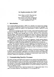
HVAC BESTEST: E300 June 28 Hourly EDB & EWB 29 27
EDB Temperature (°C)
25 23 21 19
EWB
17 15 1
2
3
4
5
6
7
8
9
10 11 12 13
14
15
16
17
18
19
20 21 22 23 24
Hour EDB:TRNSYS/TUD
EDB:DOE-2.2/NREL
EDB:DOE-2.1E-E/NREL
EDB:ENERGY+/GARD
EDB:CODYRUN/UR
EDB:HOT3000/NRCan
EDB:CO-SIMULATION
EWB:TRNSYS/TUD
EWB:DOE-2.2/NREL
EWB:DOE-2.1E-E/NREL
EWB:ENERGY+/GARD
EWB:CODYRUN/UR
EWB:HOT3000/NRCan
EWB:CO-SIMULATION
Figure 4: Zone (evaporator entering) dry-bulb (EDB) and wet-bulb (EWB) temperature for a specific simulation day.
Comparison of mono- and co-simulation Another approach to validate the coupling would be to compare results obtained by co-simulation to results obtained by mono-simulation. However, the difference in results between the mono- and the cosimulation, using different tools, would be caused not only by the coupling, but also by differences in the models and solution techniques used in the coupled simulators. To avoid errors caused by different models, only one simulator was used for both the mono- and the co-simulation. The specifications of the system can be found in Trcka (2008). Using a time step of one minute for both the mono- and the co-simulation, the difference between the results is negligible (Figure 5). With larger time steps, the influence of the time lagging of the coupling data is more noticeable. To illustrate this, the resulting zone temperatures from mono- and co-simulation, obtained using a time step of 30 minutes, are also presented in Figure 5. 30
Zone temperature [oC]
be used. HVAC BESTEST Volume 1 considers steady state tests that can be solved with analytical solutions. Volume 2 includes hourly dynamic effects and other physical phenomena that cannot be solved analytically. It has been used to validate several state of the art BPS tools. However, even though BESTEST Volume 2 has been used to validate EnergyPlus, the standard TRNSYS version (used in the prototypes) has been validated using only Volume 1 cases (Kummert et al. 2004). HVAC BESTEST Volume 2 cases were used to validate a custom version of TRNSYS that includes new code developed by the Technische Universität Dresden (TUD). Thus, the coupling could not be validated using the traditional BPS validation procedures. However, as a preliminary validation test, the HVAC BESTEST E300 case was used with the available TRNSYS models, which have not been previously validated. For the preliminary assessment of the validity of the coupling implemented in the prototypes, the reference case - E300 - from the HVAC BESTEST Volume 2 was used. To reduce any potential modelling error, the zone model was taken from the original EnergyPlus model of E300. The system was modelled using TRNSYS Type 665. The results are compared against the results obtained by different BPS programs. The co-simulation model of the case HVAC BESTEST E300 with EnergyPlus and TRNSYS cannot be used with an ideal system control for the following two reasons. First, the system modelled in TRNSYS has an ON/OFF control and not a continuous control. Second, co-simulation does not allow the distributed ideal control modelling. Thus, a model of a realistic controller was used. However, using the realistic controller with the fast responding building with low-capacitance envelope and steady state HVAC system model results in oscillatory zone temperatures even for small time steps. Consequently, the co-simulation model does not exactly replicate the E300 model requirements, which should be taken into account when comparing the results. The simulations were performed using inter-domain system decomposition and loose coupling. The temperatures of one-day simulation are shown in Figure 4. Similar results were obtained for loads and humidity ratios. The simulation was performed with a time step of one minute and the shown results are hourly averaged values. The figure shows good agreement between the co-simulation results and the results obtained by other tested BPS programs.
25
20
15
MONO-SIM (50%REC;50%AMB) - 1min
10
CO-SIM (50%REC;50%AMB) - 1min MONO-SIM (50%REC;50%AMB) - 30min
5
CO-SIM (50%REC;50%AMB) - 30min 0 0
2
4
6
8
10
12
14
16
18
20
22
24
Time [h]
Figure 5: Temperature trajectories obtained by mono- and co-simulation with ∆t=1min and ∆t=30min.
Comparison of different co-simulation implementations The implementations of loose and strong coupling, and of intra- and inter-domain decomposition, are independent of each other. A comparison of results
- 728 -
summary, with respect to computation time and ease of implementation, we recommend the loose coupling strategy with small time steps. Next, we analyzed accuracy vs. computation time. To measure accuracy, we computed the root mean square of the difference in the zone temperature and the reference zone temperature, which was obtained with strong coupling and a time step of one minute. The simulations were performed using inter-domain decomposition and loose coupling. Figure 7 shows the accuracy vs. computation time. The computation time was measured using the wall-clock time from the time point when shared memory has been initiated to the time point when the calculations finished.
obtained by different implementations was done to increase confidence in co-simulation. The specifications of the system used in the validation are described in Trcka (2008). 32
Intra Decomp; Strong Coupl Intra Decomp; Loose Coupl 30
Inter Decomp; Strong Coupl
Zone temperature [oC]
Inter Decomp; Loose Coupl 28
26