IEEE TRANSACTIONS ON SYSTEMS, MAN, AND CYBERNETICS—PART C: APPLICATIONS AND REVIEWS, VOL. 31, NO. 4, NOVEMBER 2001
497
Learn++: An Incremental Learning Algorithm for Supervised Neural Networks Robi Polikar, Member, IEEE, Lalita Udpa, Senior Member, IEEE, Satish S. Udpa, Senior Member, IEEE, and Vasant Honavar
Abstract—We introduce Learn++, an algorithm for incremental training of neural network (NN) pattern classifiers. The proposed algorithm enables supervised NN paradigms, such as the multilayer perceptron (MLP), to accommodate new data, including examples that correspond to previously unseen classes. Furthermore, the algorithm does not require access to previously used data during subsequent incremental learning sessions, yet at the same time, it does not forget previously acquired knowledge. Learn++ utilizes ensemble of classifiers by generating multiple hypotheses using training data sampled according to carefully tailored distributions. The outputs of the resulting classifiers are combined using a weighted majority voting procedure. We present simulation results on several benchmark datasets as well as a real-world classification task. Initial results indicate that the proposed algorithm works rather well in practice. A theoretical upper bound on the error of the classifiers constructed by Learn++ is also provided. Index Terms—Catastrophic forgetting, classification algorithms, ensemble of classifiers, incremental learning, knowledge acquisition and retention, pattern recognition, supervised neural networks.
I. INTRODUCTION
M
ACHINE LEARNING offers one of the most cost effective and practical approaches to the design of pattern classifiers for a broad range of pattern recognition applications. The performance of the resulting classifier relies heavily on the availability of a representative set of training examples. In many practical applications, acquisition of a representative training data is expensive and time consuming. Consequently, it is not uncommon for such data to become available in small batches over a period of time. In such settings, it is necessary to update an existing classifier in an incremental fashion to accommodate new data without compromising classification performance on old data. Learning new information without forgetting previously acquired knowledge, however, raises the so-called stability–plasticity dilemma [1], one of the fundamental problems in knowledge management (KM): Some information may have
Manuscript received June 1, 2001; revised October 1, 2001. R. Polikar is with the Department of Electrical and Computer Engineering, Rowan University, Glassboro, NJ 08028 USA (e-mail:
[email protected]). L. Udpa is with the Department of Electrical and Computer Engineering, Iowa State University, Ames, IA 50011 USA (e-mail:
[email protected]). S. S. Udpa is with the Department of Electrical and Computer Engineering, Michigan State University, East Lansing, MI 48824 USA (e-mail:
[email protected]). V. Honavar is with the Artificial Intelligence Research Laboratory, Department of Computer Science, Iowa State University, Ames, IA 50011 USA (e-mail:
[email protected]). Publisher Item Identifier S 1094-6977(01)11261-7.
to be lost to learn new information, as learning new patterns will tend to overwrite formerly acquired knowledge. The dilemma points out the fact that a completely stable classifier will preserve existing knowledge, but will not accommodate any new information, whereas a completely plastic classifier will learn new information but will not conserve prior knowledge. A typical approach for learning new information involves discarding the existing classifier, and retraining the classifier using all of the data that have been accumulated thus far. Examples of this approach include common neural network (NN) paradigms, such as multilayer perceptron (MLP), radial basis function (RBF) networks, wavelet networks, and Kohonen networks. This approach, lying on the “stability” end of the spectrum, however, results in loss of all previously acquired information, which is known as catastrophic forgetting. Furthermore, this approach may not even be feasible in many applications, particularly if the original data is no longer available. An alternative approach, lying toward the “plasticity” end of the spectrum, involves the use of online training algorithms. However, many existing online algorithms assume rather restricted form of classifiers, such as classifiers that compute conjunctions of Boolean features. Consequently, such algorithms have limited applicability in real-world applications. A third approach to incremental learning is the use of instance-based learners such as nearest neighbor classifiers. However, this approach entails storing all of the data. Various algorithms suggested in the literature for incremental learning typically use one or a combination of the above-mentioned approaches, and fall somewhere in between the stability–plasticity spectrum. Some of the more recent and prominent of such algorithms are discussed in the next section. We should also note that the term “incremental learning” has been used rather loosely in the literature, where the term referred to as diverse concepts as incremental network growing and pruning, on-line learning, or relearning of formerly misclassified instances. Furthermore, various other terms, such as constructive learning, lifelong learning, and evolutionary learning have also been used to imply learning new information. Against this background, precise formulations of the incremental learning problem, characterizations of information requirements of incremental learning, and the establishment of necessary and sufficient conditions for incremental learning need to be established. In this paper, we therefore define an incremental learning algorithm as one that meets the following criteria: 1) It should be able to learn additional information from new data.
1094–6977/01$10.00 © 2001 IEEE
498
IEEE TRANSACTIONS ON SYSTEMS, MAN, AND CYBERNETICS—PART C: APPLICATIONS AND REVIEWS, VOL. 31, NO. 4, NOVEMBER 2001
2) It should not require access to the original data, used to train the existing classifier. 3) It should preserve previously acquired knowledge (that is, it should not suffer from catastrophic forgetting). 4) It should be able to accommodate new classes that may be introduced with new data. An algorithm that possesses these properties would be an indispensable tool for pattern recognition and machine learning researchers, since virtually unlimited number of applications can benefit from such a versatile incremental learning algorithm. The problem addressed in this paper is therefore designing a supervised incremental learning algorithm satisfying all of the above-mentioned criteria. The rest of this paper is organized as follows. In Section II, we provide an overview of various approaches suggested for incremental learning algorithms, as well as an overview of ensemble-based learning algorithms, which were originally proposed for improving generalization performance of classifiers. In Section III, we show how ensemble-based approaches can be used in an incremental learning setting, and present the Learn++ algorithm in detail. In Section IV, we explain the benchmark and real-world databases used to evaluate the algorithm, along with simulation results obtained on these databases. We also compare the Learn++ performance to that of fuzzy ARTMAP on the real-world database. Finally, in Section V, we summarize our conclusions and point at future research directions. II. BACKGROUND A. Incremental Learning As mentioned earlier, various algorithms have been suggested for incremental learning, where incremental learning implied different problems. For example, in some cases, the phrase “incremental learning” has been used to refer to growing or pruning of classifier architectures [2]–[4] or to selection of most informative training samples [5]. In other cases, some form of controlled modification of classifier weights has been suggested, typically by retraining with misclassified signals [6]–[12]. These algorithms are capable of learning new information; however, they do not simultaneously satisfy all of the above-mentioned criteria for incremental learning: they either require access to old data, forget prior knowledge along the way, or unable to accommodate new classes. One notable exception is the (fuzzy) ARTMAP algorithm [13], [14], which is based on generating new decision clusters in response to new patterns that are sufficiently different from previously seen instances. This sufficiency is controlled by a user-defined vigilance parameter. Each cluster learns a different hyper-rectangle shaped portion of the feature space in an unsupervised mode, which are then mapped to target classes. Since previously generated clusters are always retained, ARTMAP does not suffer from catastrophic forgetting. Furthermore, ARTMAP does not require access to previously seen data, and it can accommodate new classes. Therefore, ARTMAP fits perfectly into our description of incremental learning. ARTMAP is a very powerful and versatile algorithm; however, it has its own drawbacks. In many applications, researchers have noticed that ARTMAP is very sensitive to selection of the
vigilance parameter, to the noise levels in the training data and to the order in which the training data is presented to the algorithm. Furthermore, the algorithm generates a large number of clusters causing overfitting, resulting in poor generalization performance, if the vigilance parameter is not chosen correctly. Therefore, this parameter is typically chosen in an ad hoc manner by trial and error. Various algorithms have been suggested to overcome such difficulties [15]–[20]. Other incremental learning algorithms, such as incremental construction of support vector machine classifiers with provable performance guarantees [21], incremental learning based on reproducible kernel Hilbert spaces [22], or incrementally adding new IF–THEN rules to an existing fuzzy inference system [23] have also been suggested. These algorithms also fit to the incremental learning setting described above, however, they require either precise a priori knowledge of data distributions, or an ad-hoc selection of a large number of parameters. B. Ensemble of Classifiers In this paper, we follow a different approach to the incremental learning problem, and present an algorithm that not only satisfies all criteria mentioned above, but also overcomes the difficulties that are associated with ARTMAP and ARTMAP based classifiers. In essence, instead of generating new cluster nodes for each previously unseen (or sufficiently different) instance, we generate multiple new “weak classifiers” for previously unseen portions of the feature space. This conceptually subtle difference, allows us to develop a fundamentally different incremental learning algorithm that is insensitive to the order of presentation of the training data, or even to the minor adjustments of the algorithm parameters. Learn++, the proposed incremental learning algorithm described in the next section, was inspired by the AdaBoost (adaptive boosting) algorithm, originally developed to improve the classification performance of weak classifiers. Schapire showed that for a two class problem, a weak learner that can barely do little better than random guessing can be transformed into a strong learner that almost always achieves arbitrarily low error rate using a procedure called boosting [24]. Freund et al. later developed AdaBoost, extending boosting to multiclass and regression problems [25], [26]. In essence, both Learn++ and AdaBoost generate an ensemble of weak classifiers, each trained using a different distribution of training samples. The outputs of these classifiers are then combined using Littlestone’s majority-voting scheme [27] to obtain the final classification rule. Combining weak classifiers take advantage of the so-called instability of the weak classifier. This instability causes the classifiers to construct sufficiently different decision surfaces for minor modifications in their training datasets. The idea of generating an ensemble of classifiers for improving classification accuracy was formerly introduced by many other researchers. For example, Wolpert suggested combining hierarchical levels of classifiers, using a procedure called stacked generalization [28]. Jordan and Jacobs introduced hierarchical mixture of experts (HME), where multiple classifiers were highly trained (hence experts) in different regions of the feature space, and their outputs were then weighted using a gating network [29], [30]. Kitler et al. analyzed error
POLIKAR et al.: LEARN++: AN INCREMENTAL LEARNING ALGORITHM
sensitivities of various voting and combination schemes [31], whereas Rangarajan et al. investigated the capacity of voting systems [32]. Ji and Ma proposed an alternative approach to AdaBoost that generates simple perceptrons of random parameters and then combines the perceptron outputs using majority voting [33], similar to generating an ensemble of classifiers through randomizing the internal parameters of a base classifier, previously introduced by Ali and Pazzani [34]. Ji and Ma give an excellent review of various methods for combining classifiers in [35], whereas Dietterich compares ensemble of classifiers to other types of learners, such as reinforcement and stochastic learners in [36]. There have also been some attempts for using HMEs in an online setting to incrementally learn from incoming data [30], [37], however such attempts have not addressed all of the above mentioned issues of incremental learning, in particular, learning new classes. Consequently, research on combining classifiers have been mostly limited to improving performance of classifiers, rather than incremental learning. This leads us to consider adaptations of ensemble-based methods such as AdaBoost or HME to achieve incremental learning. III. ENSEMBLE OF CLASSIFIERS FOR INCREMENTAL LEARNING: LEARN++ Combining ensemble of classifiers in Learn++ is specifically geared toward achieving incremental learning, as described by the criteria mentioned earlier. However, due to their similarities, Learn++ also inherits performance improvement properties of AdaBoost, as shown in simulation results. Learn++ is based on the following intuition: Each new classifier added to the ensemble is trained using a set of examples drawn according to a distribution, which ensures that examples that are misclassified by the current ensemble have a high probability of being sampled. In an incremental learning setting, the examples that have a high probability of error are precisely those that are unknown or that have not yet been used to train the classifier. As mentioned earlier, both AdaBoost and Learn++ generate weak hypotheses and combine them through weighted majority voting of the classes predicted by the individual hypotheses. The hypotheses are obtained by retraining a base classifier (weak learner) using strategically updated distributions of the training database. AdaBoost’s distribution update rule is optimized for improving classifier accuracy, whereas Learn++ distribution update rule is optimized for incremental learning of new data, in particularwhenthenewdataintroducesnewclasses.Intheinterest of space, only Learn++, and its major differences from AdaBoost are given below.Details ofAdaBoost canbefoundin [25]. The Learn++ algorithm is given in Fig. 1. Inputs to Learn++ are , 1) training data are training instances and are the correwhere samples sponding correct labels for database ; randomly selected from the 2) a weak learning algorithm WeakLearn, to be used as the base classifier; 3) an integer , specifying the number of classifiers to be generated.
499
Recall that a weak learning algorithm is used as a base classifier, to allow sufficiently different decision boundaries to be generated by slightly modified training datasets. Also note that most strong classifiers spend a majority of their training time in fine-tuning the decision boundary. As described below, Learn++ requires each weak learner to generate only a rough estimate of the actual decision boundary, effectively eliminating the costly fine-tuning step, allowing faster training and less over fitting. Each classifier can be thought of as a hypothesis from the input space to the output space . Learn++ asks WeakLearn to generate multiple hypotheses using different subsets of the training data , and each hypothesis learns only a portion of the input space. This is achieved by iteratively updating a distribution , from which training subsets are chosen. The distribution itself is obtained by normalizing a set of weights assigned to each instance based on the classification performance of the classifiers on that instance (Step 1). In general, instances that are difficult to classify receive higher weights to increase their chanceofbeingselectedintothenexttrainingdataset.Theweights for the first iteration are initialized to , giving equal likelihood to each instance to be selected into the first training subset, unless there is sufficient reason to initialize otherwise. , Learn++ first diAt each iteration into a training subset and a test subset chotomizes according to the current distribution (Step 2), and calls WeakLearn to generate the hypothesis (Step 3) using the training subset . The error of on is defined as (Step 4) (1) which is simply the sum of distribution weights of misclassified , is discarded and new and instances. If are selected. That is, the weak hypothesis is only expected to achieve a 50% (or better) empirical classification performance on the . For a binary class problem, this is the least restrictive requirement one could have, since an error of one-half for a binary class problem means random guessing. However, obtaining a maximum error of one-half becomes increasingly difficult as the number of classes increase, since for an class problem, the . Therefore, error generated by random guessing is the choice of a weak learning algorithm with a minimum classification performance of 50% may not be trivial. However, NN algorithms can easily be configured to simulate weak learners, by modifying their size and error goal parameters. Use of strong learners, on the other hand, are not recommended in algorithms using the ensemble of classifiers approach, since there is little to be gained from their combination, and/or they may lead to over fitting of the data [25], [35]. is satisfied, then the normalized error If, is computed as (2) All hypotheses generated in the previous iterations are then combined using weighted majority voting (Step 5). The voting weights are computed as the logarithms of the reciprocals of normalized errors . Therefore, those hypotheses that perform
500
IEEE TRANSACTIONS ON SYSTEMS, MAN, AND CYBERNETICS—PART C: APPLICATIONS AND REVIEWS, VOL. 31, NO. 4, NOVEMBER 2001
Fig. 1. Algorithm Learn++.
well on their own training and test data are given larger voting powers. A classification decision is then made based on the combined outputs of individual hypotheses, which constitutes the composite hypothesis (3)
decides on the class that receives the highest Note that total vote from all hypotheses. The composite error made by is then computed as (4)
on misclassified instances, where is 1 if the predicate is , current is discarded, a true, and 0 otherwise. If is generated. We new training subset is selected and a new note that can only exceed this threshold during the immediate is introduced. At all other iteration after a new database will be satisfied, since all hypotheses that times, make up the composite hypothesis have already been verified in Step 4 to achieve a minimum of 50% performance on . If , composite normalized error is computed as (5) are then updated, for computing the next The weights , which in turn is used in selecting the next distribution training and testing subsets, and , respectively.
POLIKAR et al.: LEARN++: AN INCREMENTAL LEARNING ALGORITHM
501
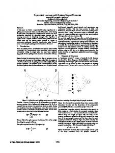
The distribution update rule constitutes the heart of the algorithm, as it allows Learn++ to learn incrementally if otherwise (6) is correctly classified According to this rule, if instance , its weight is multiplied by a by the composite hypothesis factor of , which, by its definition, is less than 1. If is misclassified, its distribution weight is kept unchanged. This rule reduces the probability of correctly classified instances being , while increasing the probability of misclaschosen into . If we interpret insified instances to be selected into stances that are repeatedly misclassified as hard instances, and those that are correctly classified as simple instances, the algorithm focuses more and more on hard instances, and forces additional classifiers to be trained with them. Instances coming from previously unseen parts of the feature space, such as those from new classes, can be interpreted as hard instances at the time they are introduced to the algorithm. Note that using the composite hypothesis in (6) makes incremental learning possible particularly when instances from new classes are introduced, since these instances will be misclassified by the composite hypothesis and forced into the next training dataset. The procedure would not work nearly as efficiently, if the weight update rule were based on the performance of the previous only (as AdaBoost does) instead of the composite hypothesis . Apart from the distribution update rule, Learn++ also differs from AdaBoost in definition of training error and the evaluation of individual hypotheses. During each iteration, Learn++ generates on which the training error and an additional test subset hypothesis evaluation are based, whereas AdaBoost computes the individual hypothesis errors on their own training data only. Finally, since AdaBoost does not compute a composite hypothesis, composite error is also not applicable in AdaBoost. hypotheses are generated for each database , the After final hypothesis is obtained by the weighted majority voting of all composite hypotheses (7) Note that while incremental learning is achieved through generating additional classifiers, former knowledge is not lost, since all classifiers are retained. Another important property of Learn++ is its independence of the base classifier used as a weak learner. In particular, it can be used to convert any supervised classifier, originally incapable of incremental learning, to one that can learn from new data. Fig. 2 conceptually illustrates Learn++ architecture on an example. The dark curve is the decision boundary to be learned and the two sides of the dashed line represent the and , which need feature space for two training databases not be mutually exclusive. Weak hypotheses are illustrated with simple geometric figures, generated by weak learners , where through are generated through due to training with different subsets of , and
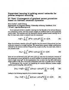
are generated due to training with different subsets of . Hypotheses decide whether a data point is within the decision boundary. They are hierarchically combined to form composite , which are then combined to form hypotheses . the final hypothesis Learn++ guarantees convergence on any given training dataset, by reducing the classification error with each added hypothesis. We state the theorem that relates the overall upper error bound of Learn++ to individual errors of each hypothesis, the proof of which is given in the Appendix. Theorem: The training error of the Learn++ algorithm given , in Fig. 1 is bounded above by is the error of the th composite hypothwhere . Furthermore, is itself bounded above by esis , where is the error of the individual hypothesis . IV. EXPERIMENTS WITH LEARN++ The algorithm was tested on various benchmark and real-world databases. Due to space limitations, results on four databases are presented here, with additional results available on the web [38]. Detailed descriptions of each database along with the performance of the algorithm on these databases are explained in the following sections. In all experiments, previously seen data were not used in subsequent stages of learning, and in each case the algorithm was tested on an independent validation dataset that was not used during training. In all cases, we have used a relatively small MLP trained with a large error goal as the base classifier to simulate a weak learner. We note that Learn++ itself is independent of the classifier used. MLP was used since it is the most commonly employed classification algorithm that is not capable of incremental learning without catastrophic forgetting. Different architectures and error goals were tried to test the algorithm’s sensitivity and invariance to minor modifications to parameter selections, including the MLP architecture, mean square error (MSE) goal, and the number of hypotheses generated. The parameters given below are typical representatives of those that have been tried. Furthermore, in order to test the sensitivity of Learn++ to the order of presentation of the data, multiple experiments were performed for all databases, where the order of the datasets introduced to the algorithm at different times were varied. The results for all cases were virtually the same. Average representative performance results are presented below. A. Optical Digits Database This benchmark database, obtained from the UCI machine learning repository [39], consisted of 5620 instances of digitized handwritten characters; 1200 instances were used for training and all remaining instances were used for validation. The characters were numerals 0–9, and they were digitized on grid, creating 64 attributes. This dataset was used to an evaluate Learn++ on incremental learning without introducing new classes. Fig. 3 shows sample images of this database. The training dataset of 1200 instances were divided into six subsets, , each with 200 instances containing all ten classes
502
Fig. 2.
IEEE TRANSACTIONS ON SYSTEMS, MAN, AND CYBERNETICS—PART C: APPLICATIONS AND REVIEWS, VOL. 31, NO. 4, NOVEMBER 2001
Combining classifiers for incremental learning.
to be used in six training sessions. In each training session, only one of these datasets was used. For each training session , 30 weak hypotheses were generated by of the th Learn++. Each hypothesis and training session was generated using a training subset (used to compute hypothesis error), each a testing subset with 100 instances drawn from . The base classifier was a single hidden layer MLP with 30 hidden layer and ten output nodes with a MSE goal of 0.1. An additional validation set, TEST, of 4420 instances was used for validation purposes. Note that NNs can simulate a weak learner, when their architecture is kept small and their error goal is kept high with respect to the complexity of the particular problem. The relatively high error goal of 0.1 allowed the MLP to serve as a weak learner in this case, as shown in the Average/learner column of Table I, which indicates the average performance of individual . On average, weak learners hypotheses on each database performed little over 50%, which improved to over 90% when the hypotheses were combined. This improvement demonstrates the performance improvement property of Learn++ (as inherited from AdaBoost) on a given single database. Each column thereafter indicates Learn++ performance on the current and previous training datasets as additional data were introduced. Previous datasets were not used for training in subsequent training sessions, but they were only used to evaluate the algorithm performance on previously seen instances to make sure that previously acquired knowledge was not lost. The last row of Table I shows the classification performance on the validation dataset, which gradually and consistently improved from 82% to 93% as new databases became available, demonstrating the incremental learning capability of the proposed algorithm. In order to compare the performance of Learn++ to that of a strong learner trained with the entire training data of 1200 instances, various architecture–error goal combinations were tried. An MLP with 50 hidden layer nodes and a 100 times smaller error goal of 0.001 was able to match (and slightly exceed) Learn++ performance, by classifying 95% of the TEST dataset. B. Vehicle Silhouette Database Also obtained from the UCI depository, the vehicle silhouette database consisted of 18 features from which the type of a vehicle is determined. The database consisted of 846 instances, of 210 which was divided into three training datasets instances each, and a validation dataset, TEST, of 216 instances , 30 hyin four classes. For each training session
Fig. 3. Sample images from the optical digits database.
potheses were generated using a 30-node single hidden layer MLP with an error goal of 0.1. This particular benchmark database is considered as one of the more difficult databases in the repository, since generalization performances using various algorithms (strong learners) have been in the 65%–80% range [40], [41]. The results are presented in Table II, where the Average/learner column indicates the average performance of a weak hypothesis (a single MLP). We note from the average 62% performance that the chosen MLP architecture and error goal was able to simulate a weak learner. The other columns indicate the Learn++ performance on individual training datasets and on the validation dataset after each of the three training sessions. As seen in Table II, there is a minor and gradual loss of information on the previous training datasets as new datasets are introduced, however, the generalization performance on the validation dataset improved from 78% to 83%. This performance was comparable, or better, than the performance of most algorithms that were trained using the entire data [41]. C. Concentric Circles Database This rather simple synthetic database of concentric rings with two attributes and five classes was generated for testing Learn++ performance on incremental learning when new classes are introduced. Fig. 4 illustrates this database. The database was dithrough , and a validavided into six training datasets, and had 50 instances from each of tion dataset TEST. and had 50 instances the classes 1, 2, and 3; datasets had from each of the classes 1, 2, 3, and 4; and datasets 50 instances from each of the classes 1–5. The validation set TEST had 500 instances from all five classes. Table III presents the classification performance results. The validation on TEST dataset shows steadily increasing generalization performance, indicating the algorithm was able to learn the new information, and the new classes, successfully. Note that larger improvements in the performance are obtained after the third and fifth training sessions, since these training sessions introduced new
POLIKAR et al.: LEARN++: AN INCREMENTAL LEARNING ALGORITHM
503
TABLE I TRAINING AND GENERALIZATION PERFORMANCE OF LEARN++ ON OPTICAL DIGITS DATABASE
TABLE II TRAINING AND GENERALIZATION PERFORMANCE OF LEARN++ ON VEHICLE DATABASE
tally, to test the algorithm’s sensitivity to the order of presentation of the data. The results, which are provided on the web [38], were virtually the same. Finally, in order to compare the incremental learning performance of Learn++ to that of a strong learner trained on the entire training data, a larger MLP with 50 hidden nodes and an error goal of 0.005 was trained. The performance of this strong learner was 95%, only slightly better than that of Learn++. D. Gas Sensing Dataset
Fig. 4.
Circular regions database.
classes that were not available earlier. Similarly, the improvements in the performance after the fourth and sixth training sessions are minor compared to the previous sessions, since these sessions did not introduce new classes. This is also reflected in the number of hypotheses generated during each training session, which are given in parentheses on the first row of the table. Note that when new classes are introduced, the number of hypotheses generated in each session is not the same. The number of hypotheses generated was determined simply by monitoring the classification performance, where each training session was terminated when the performance no longer improved. The last column titled “Last 7” indicates the Learn++ performance on the last seven hypotheses. Although these hypotheses were trained with a dataset that included all classes, they were not adequate to give satisfactory performance, demonstrating that all hypotheses are required for the final classification. An alternative set of six datasets was also generated from this database, by changing the order of classes introduced incremen-
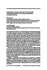
Learn++ was then implemented on real-world data obtained from a set of six polymer-coated quartz crystal microbalances (QCMs) used to detect volatile organic compounds (VOCs). Detection and identification of VOCs are of crucial importance for environmental monitoring and in gas sensing. Piezoelectric acoustic wave sensors, which comprise a versatile class of chemical sensors, are used for the detection of VOCs. For sensing applications, a sensitive polymer film is cast on the surface of the QCM. This layer can bind a VOC of interest, altering the resonant frequency of the device, in proportion to the added mass. Addition or subtraction of gas molecules from the surface or bulk of an acoustic wave sensor results in a change in its resonant frequency. The frequency change , caused by a deposited mass can be described by where is the fundamental is the active resonant frequency of the bare crystal, and surface area [42]. The sensor typically consists of an array of several crystals, each coated with a different polymer. This design is aimed at improving identification, hampered by the limited selectivity of individual films. Employing more than one crystal, and coating each with a different partially selective polymer, different responses can be obtained for different gases. The combined response of these crystals can then be used as a signature pattern of the VOC detected. The gas sensing dataset used in this study consisted of responses of six QCMs to five VOCs, including ethanol (ET), xylene (XL), octane (OC), toluene (TL), and trichloroethelene (TCE). Fig. 5 illustrates sample patterns for each VOC from
504
IEEE TRANSACTIONS ON SYSTEMS, MAN, AND CYBERNETICS—PART C: APPLICATIONS AND REVIEWS, VOL. 31, NO. 4, NOVEMBER 2001
TABLE III TRAINING AND GENERALIZATION PERFORMANCE OF LEARN++ ON CONCENTRIC CIRCLES DATABASE
Fig. 5.
Sample responses of the six-QCM sensor array to VOCs of interest. TABLE IV DATA-CLASS DISTRIBUTION FOR THE GAS SENSING DATABASE
six QCMs coated with different polymers, where the vertical axis represents normalized frequency change. Note that the patterns from toluene, xylene, and TCE look considerably similar; hence, they are difficult to distinguish from each other. Further details on VOC recognition using QCMs can be found in [42], whereas more information on this dataset, experimental setup for generating the gas sensing signals, and sample patterns are provided on the web [43]. The dataset consisted of 384 six-dimensional patterns, half of which were used for training. Table IV presents the distribution of the datasets, where subsequent datasets are strongly biased toward the new class. Such a distribution results in an even tougher challenge; since the algorithm will no longer have the opportunity to see adequate number of instances from previously introduced classes in the subsequent training sessions. The performance of Learn++ on this dataset is shown in Table V. The generalization performance of Learn++ on the validation dataset, gradually improving from 61% to 88% as new data was introduced, demonstrates its incremental learning capability even when instances of new classes are introduced in subsequent training sessions. Learn++ performance on this dataset was comparable to that of a strong learner, a two hidden layer MLP of error goal 0.001, trained with the entire training data, which had a classification performance of 90%. Learn++ was able to perform as well as the strong learner, by seeing only a portion of
the dataset at a time. This dataset was also presented to the algorithm in a different order, and the resulting performances were virtually the same, implying that the algorithm is not sensitive to the order of presentation of the training data. Furthermore, various minor modifications to the base classifier architecture nodes) and error goal ( ) also resulted in ( similar performances, indicating that the algorithm is not very sensitive to minor changes in its parameters. A formal analysis on how much such parameters can be changed without affecting the performance is currently underway. Finally, Learn++ was also compared to fuzzy ARTMAP on this database. Table VI presents the performance figures of fuzzy ARTMAP on the identical dataset described in Table IV for various values of the vigilanceparameter .The classification performance of fuzzy ARTMAP is always 100% on training data, since according to the ARTMAP learning algorithm, convergence is achieved only when all training data are correctly classified. Furthermore, once a pattern is learned, a particular cluster is assigned to it, and future training does not alter this clustering. Therefore, ARTMAP never forgets what it has seen as a training data instance. The improvement in the classification performance of the testdataonceagaindemonstratesthatARTMAPisindeedcapable of incremental learning. However, fuzzy ARTMAP was indeed sensitive to slight changes in its vigilance parameter, and even its was about 5% points less best performance of 83.8% for that than of Learn++. V. SUMMARY AND DISCUSSION This paper introduced Learn++, a versatile incremental learning algorithm based on synergistic performance of an ensemble of weak classifiers/learners. Learn++ can learn from new data even when the data introduces new classes.
POLIKAR et al.: LEARN++: AN INCREMENTAL LEARNING ALGORITHM
TRAINING
AND
TABLE V GENERALIZATION PERFORMANCE GAS SENSING DATABASE
OF
LEARN++
ON
TABLE VI FUZZY ARTMAP PERFORMANCE ON THE GAS SENSING DATABASE
Learn++ does not require access to previously used data during subsequent training sessions, and it is able to retain previously acquired knowledge. Learn++ makes no assumptions as to what kind of weak learning algorithm is to be used. Any weak learning algorithm can serve as the base classifier of Learn++, though the algorithm is optimized for supervised NN-type classifiers, whose weakness can be easily controlled via network size and error goal. Learn++ is also intuitively simple, easy to implement, and converges much faster than strong learning algorithms. This is because using weak learners eliminates the problem of finetuning and over fitting, since each learner only roughly approximates the decision boundary. Initial results using this algorithm look promising, but there is significant room for improvement and many questions to be answered. The algorithm has two key components, both of which can be improved. The first one is the selection of the subsequent training dataset, which depends on the distribution update rule. AdaBoost depends solely on the performance of individual , for distriwhereas Learn++ uses the performance of overall bution update. The former guarantees robustness and prevents performance deterioration, whereas the latter allows efficient incremental learning capability when new classes are introduced. An appropriate combination of the two updating schemes might provide optimum performance levels. Initialization of the distribution when a new database is introduced can also be optimized by an initial classification evaluation of the composite hypotheses on the new database. The second key factor in Learn++ is the hypothesis combination rule. Currently, voting weights are determined based on performances of the hypotheses on their own training data subset. This is suboptimal, since the performance of a hypothesis on a specific subset of the input space does not guarantee the performance of that hypothesis on an unknown instance, which may come from a different subset of the space. This static combination rule can be replaced by a dynamic rule that estimates which hypotheses are likely to correctly classify a given (unknown) in-
505
stance, based on statistical distance metrics or a posteriori probabilities, and determine voting weights accordingly for each instance. Other issues include selection of algorithm parameters, and using other classifiers as weak learners. The algorithm parameters, such as base classifier architecture, error goal, number of hypotheses to be generated, are currently chosen in a rather ad hoc manner. Although the algorithm appears to be insensitive to minor changes in these parameters, a formal method for selecting them would be beneficial. Future work will also include evaluating Learn++ with other classifiers used as weak learners, such as RBF NNs and non-NN-based classification/clustering algorithms. Finally, the weighted majority voting for combining the hypotheses hints at a simple way of estimating the reliability of the final decision and confidence limits of the performance figures. In particular, if a vast (marginal) majority of agree on the class of a particular instance, then this can be interpreted as the algorithm having high (low) confidence in the final decision. A formal analysis of classifier reliability and confidence intervals of the classifier outputs can be done by computing a posteriori probabilities of classifier outputs, which can then be compared to those obtained by using vote count mechanism. APPENDIX ERROR BOUND ANALYSIS FOR LEARN++ Theorem: The training error of the Learn++ algorithm given , in Fig. 1 is bounded above by is also bounded above by the AdaBoost.M1 error where . bound Proof: Following a similar approach given in [25], we first show that the above error bound holds for a two-class problem, and then show that a multiclass problem can be reduced to a binary class problem, allowing the same error bound to hold for the multiclass case as well. Let us call the algorithm working on binary problems Learn+ (as opposed to Learn++, which is reserved for the multiclass problem). In a binary class setting where the two possible values for are 0 and 1, the equations for error terms and distribution update rules given in Fig. 1 can be simplified as follows. The combined hypothesis is obtained by if otherwise whereas the error for
(8)
is (9)
the distribution update rule is given by if otherwise (10)
506
IEEE TRANSACTIONS ON SYSTEMS, MAN, AND CYBERNETICS—PART C: APPLICATIONS AND REVIEWS, VOL. 31, NO. 4, NOVEMBER 2001
Hence,
and the final classification rule for each dataset is
(19)
if
(11)
otherwise. We define the error of the final hypothesis as sum of the initial weights of the misclassified instances, that is (12) To find and upper bound for , we analyze the final weights of the instances after iterations, and associate these weights . Note with the errors committed by combined hypotheses that after rounds, the final weight for any instance is
giving us an upper bound for the error of the final hypothesis. However, this upper bound based on the weights of individual instances is of little use, since it is difficult to keep track of the weights of every instance used for each hypothesis. These sum of weights can also be limited by an upper bound, based on the for errors of each . Recognizing that , and starting with the sum of the weights of all instances
(13)
(20)
(14)
We now define the intermediate variable as the loss of the th hypothesis on instance , then the total error of the th combined hypothesis is
The summation over all instances gives
Comparing the sum of weights of all instances to the sum of the weights that are misclassified
(21) (15) We now note that the final hypothesis take on instance if and only if
Furthermore, recall from Step 1 of Learn++ algorithm that
will make a mis-
(22) Substituting (21) and (22) into (20), we obtain
(16) or alternatively, if and only if (17) Incorporating (17) into (15) for misclassified instances, we obtain from (22), we obtain
(18)
POLIKAR et al.: LEARN++: AN INCREMENTAL LEARNING ALGORITHM
507
and from (21)
(23) After
iterations, we obtain (24)
Substituting (24) into (19), we obtain
and . We also define the initial distribution for Learn+ instances to be the same as Learn++ instances. we pass the hypothesis For each iteration as if WeakLearn returns it to Learn+. Note that according to this formulation, if Learn++ misclassifies , . Since the correct class of the then it will return 1 to corresponding is 0, (all instances for Learn+ are of class 0 by misclassifies this instance our previous definition), then as well. On the other hand, if Learn++ correctly classifies , and since this is also the instance , it will return 0 to also classifies the correct class for all Learn+ instances, correctly. In other words, when the corresponding instance multiclass algorithm makes an error, the binary class algorithm makes an error, and when the multiclass algorithm correctly classifies an instance, so does the binary class algorithm. Since initial distributions for both algorithms were defined to be identical, errors computed by both algorithms will also be , , and . Therefore, identical, hence the error of the final hypothesis will also be identical to that given in (27). REFERENCES
or (25) which gives us an upper bound on the training error in terms of the normalized error and the actual error of the combined hypotheses . Note that no relationship has been assumed beand in this derivation We now find the optimum tween value for , from (25). Since all terms in (25) are positive, we can take the derivatives individually for each
(26) Finally, substituting (26) into (25), we obtain (27) which is identical in form to that of AdaBoost, except that the errors of individual hypotheses are replaced by the errors of . Furthermore, since each combined combined hypotheses hypothesis is obtained from individual hypotheses much like the final hypothesis is obtained from the combined hypotheses, an , which identical error analysis can be carried out for each , the error of obviously will be the AdaBoost algorithm. So far, we have only shown the error bound for the binary classification problem; however, it is easy to show that the same analysis holds for multiclass problems, by establishing a one-to-one mapping between the binary class and multiclass problems. Again, following a similar approach to that in [25], , we define for each instance in the Learn++ training set with some random number, a Learn+ instance
[1] S. Grossberg, “Nonlinear neural networks: principles, mechanisms and architectures,” Neural Netw., vol. 1, no. 1, pp. 17–61, 1988. [2] E. H. Wang and A. Kuh, “A smart algorithm for incremental learning,” in Proc. Int. Joint Conf. Neural Netw., vol. 3, 1992, pp. 121–126. [3] B. Zhang, “An incremental learning algorithm that optimizes network size and sample size in one trial,” in Proc. IEEE Int. Conf. Neural Netw., 1994, pp. 215–220. [4] F. S. Osorio and B. Amy, “INSS: A hybrid system for constructive machine learning,” Neurocomput., vol. 28, pp. 191–205, 1999. [5] A. P. Engelbrecht and R. Brits, “A clustering approach to incremental learning for feedforward neural networks,” in Proc. Int. Joint Conf. Neural Netw., vol. 3, 2001, pp. 2019–2024. [6] C. H. Higgins and R. M. Goodman, “Incremental learning with rulebased neural networks,” in Proc. Int. Joint Conf. Neural Netw., vol. 1, 1991, pp. 875–880. [7] M. T. Vo, “Incremental learning using the time delay neural network,” in Proc. IEEE Int. Conf. Acoust., Speech, Signal Proces., vol. 2, 1994, pp. 629–632. [8] T. Hoya and A. G. Constantidines, “A heuristic pattern correction scheme for GRNNs and its application to speech recognition,” in Proc. IEEE Signal Proces. Soc. Workshop, 1998, pp. 351–359. [9] K. Yamauchi, N. Yamaguchi, and N. Ishii, “An incremental learning method with retrieving of interfered patterns,” IEEE Trans. Neural Netw., vol. 10, pp. 1351–1365, Nov. 1999. [10] L. Fu, “Incremental knowledge acquisition in supervised learning networks,” IEEE Trans. Syst., Man, Cybern. A, vol. 26, pp. 801–809, Nov. 1996. [11] L. Fu, H. H. Hsu, and J. C. Principe, “Incremental backpropagation learning networks,” IEEE Trans. Neural Netw., vol. 7, pp. 757–762, May 1996. [12] L. Grippo, “Convergent on-line algorithms for supervised learning in neural networks,” IEEE Trans. Neural Netw., vol. 11, pp. 1284–1299, Nov. 2000. [13] G. A. Carpenter, S. Grossberg, and J. H. Reynolds, “ARTMAP: Supervised real-time learning and classification of nonstationary data by a self organizing neural network,” Neural Netw., vol. 4, no. 5, pp. 565–588, 1991. [14] G. A. Carpenter, S. Grossberg, N. Markuzon, J. H. Reynolds, and D. B. Rosen, “Fuzzy ARTMAP: A neural network architecture for incremental supervised learning of analog multidimensional maps,” IEEE Trans. Neural Netw., vol. 3, pp. 698–713, Sept. 1992. [15] J. R. Williamson,, “Gaussian ARTMAP: A neural network for fast incremental learning of noisy multidimensional maps,” Neural Netw., vol. 9, no. 5, pp. 881–897, 1996. [16] C. P. Lim and R. F. Harrison, “An incremental adaptive network for on-line supervised learning and probability estimation,” Neural Netw., vol. 10, no. 5, pp. 925–939, 1997.
508
IEEE TRANSACTIONS ON SYSTEMS, MAN, AND CYBERNETICS—PART C: APPLICATIONS AND REVIEWS, VOL. 31, NO. 4, NOVEMBER 2001
[17] G. Tontini, “Robust learning and identification of patterns in statistical process control charts using a hybrid RBF fuzzy ARTMAP neural network,” in Proc. Int. Joint Conf. Neural Netw., vol. 3, 1998, pp. 1694–1699. [18] F. H. Hamker, “Life-long learning cell structures—Continuously learning without catastrophic interference,” Neural Netw., vol. 14, no. 4, pp. 551–573, 2000. [19] G. C. Anagnostopoulos and M. Georgiopoulos, “Ellipsoid ART and ARTMAP for incremental clustering and classification,” in Proc. Int. Joint Conf. Neural Netw., vol. 2, 2001, pp. 1221–1226. [20] S. J. Verzi, G. L. Heileman, M. Georgiopoulos, and M. J. Healy, “Rademacher penalization applied to fuzzy ARTMAP and boosted ARTMAP,” in Proc. Int. Joint Conf. Neural Netw., vol. 2, 2001, pp. 1191–1196. [21] D. Caragea, A. Silvescu, and V. Honavar et al., “Learning in open-ended environments: Distributed learning and incremental learning,” in Architectures for Intelligence, Wermter et al., Eds. New York: SpringerVerlag, 2001. [22] S. Vijayakumar and H. Ogawa, “RKHS-based functional analysis for exact incremental learning,” Neurocomput., vol. 29, pp. 85–113, 1999. [23] G. G. Yen and P. Meesad, “An effective neurofuzzy paradigm for machine condition health monitoring,” IEEE Trans. Syst., Man, Cybern. B, vol. 31, pp. 523–536, Aug. 2001. [24] R. Schapire, “Strength of weak learning,” Machine Learn., vol. 5, pp. 197–227, 1990. [25] Y. Freund and R. Schapire, “A decision theoretic generalization of on-line learning and an application to boosting,” Comput. Syst. Sci., vol. 57, no. 1, pp. 119–139, 1997. [26] R. Schapire, Y. Freund, P. Bartlett, and W. S. Lee, “Boosting the margins: A new explanation for the effectiveness of voting methods,” Ann. Stat., vol. 26, no. 5, pp. 1651–1686, 1998. [27] N. Littlestone and M. Warmuth, “Weighted majority algorithm,” Inform. Comput., vol. 108, pp. 212–261, 1994. [28] D. H. Wolpert, “Stacked generalization,” Neural Netw., vol. 5, no. 2, pp. 241–259, 1992. [29] R. A. Jacobs, M. I. Jordan, S. J. Nowlan, and G. E. Hinton, “Adaptive mixtures of local experts,” Neural Comput., vol. 3, pp. 79–87, 1991. [30] M. I. Jordan and R. A. Jacobs, “Hierarchical mixtures of experts and the EM algorithm,” Neural Comput., vol. 6, no. 2, pp. 181–214, 1994. [31] J. Kittler, M. Hatef, R. P. Duin, and J. Matas, “On combining classifiers,” IEEE Trans. Pattern Anal. Machine Intell., vol. 20, pp. 226–239, Mar. 1998. [32] S. Rangarajan, P. Jalote, and S. Tripathi, “Capacity of voting systems,” IEEE Trans. Software Eng., vol. 19, pp. 698–706, July 1993. [33] C. Ji and S. Ma, “Combination of weak classifiers,” IEEE Trans. Neural Netw., vol. 8, pp. 32–42, Jan. 1997. [34] K. M. Ali and M. J. Pazzani, “Error reduction through learning multiple descriptions,” Machine Learn., vol. 24, no. 3, pp. 173–202, 1996. [35] C. Ji and S. Ma, “Performance and efficiency: Recent advances in supervised learning,” Proc. IEEE, vol. 87, pp. 1519–1535, Sept. 1999. [36] T. G. Dietterich, “Machine learning research,” AI Mag., vol. 18, no. 4, pp. 97–136, 1997. [37] C. K. Tham, “On-line learning using hierarchical mixtures of experts,” in IEE Conf. Artificial Neural Netw., 1995, pp. 347–351. [38] R. Polikar, “Algorithms for enhancing pattern separability, feature selection and incremental learning with applications to gas sensing electronic nose systems,” Ph.D. dissertation, Iowa State Univ., Ames, Aug. 2000. [Online]. Available: http://engineering.rowan.edu/~polikar/RESEARCH/PhDdis.pdf. [39] C. L. Blake and C. J. Merz. (1998) UCI repository of machine learning databases. Dept. Inform. and Comput. Sci., Univ. of California, Irvine. [Online]. Available: http://www.ics.uci.edu/~mlearn/MLRepository.html. [40] Y. Freund and R. Schapire, “Experiments with a new boosting algorithm,” in Proc. 13th Int. Conf. Machine Learning, 1996, pp. 148–156. [41] R. Parekh, J. Yang, and V. Honavar, “Constructive neural network algorithms for pattern classification,” IEEE Trans. Neural Netw., vol. 11, pp. 436–451, Mar. 2000. [42] A. D’Amico, C. Di Natale, and E. Verona, “Acoustic devices,” in Handbook of Biosensors and Electronic Nose. Medicine, Food and the Environment, E. Kress-Rogers, Ed. Boca Raton, FL: CRC, 1997, ch. 9, pp. 197–223. [43] R. Polikar.. [Online]. Available: http://engineering.rowan.edu/~polikar/RESEARCH/VOC_Database/voc_database.html.
Robi Polikar (S’92–M’01) received the B.S. degree in electronics and communications engineering from Istanbul Technical University, Istanbul, Turkey, in 1993, and the M.S. and Ph.D. degrees, both co-majors in biomedical engineering and electrical engineering, from Iowa State University, Ames, in 1995 and in 2000, respectively. He is currently an Assistant Professor with the Department of Electrical and Computer Engineering at Rowan University, Glassboro, NJ. His current research interests include signal processing, pattern recognition, neural systems, machine learning, and computational models of learning, with applications to biomedical engineering and imaging, chemical sensing, nondestructive evaluation, and testing. He also teaches upper undergraduate and graduate level courses in wavelet theory, pattern recognition, neural networks, and biomedical systems and devices at Rowan University. Dr. Polikar is a Member of ASEE, Tau Beta Pi, and Eta Kappa Nu. Lalita Udpa (S’84–M’86–SM’91) received the M.S. and Ph.D. degrees in electrical engineering from Colorado State University, Fort Collins, in 1981 and 1986, respectively. She is currently a Professor with the Electrical and Computer Engineering Department at Iowa State University, Ames. She works primarily in the broad areas of computational modeling, signal processing, and pattern recognition with applications to nondestructive evaluation (NDE). Her research interests include development of finite element models for electromagnetic NDE phenomena, applications of neural networks and signal processing algorithms for the analysis of NDE measurements, and development of image processing techniques for flaw detection in noisy, low-contrast X-ray images. Dr. Udpa is a senior member of Sigma Xi and Eta Kappa Nu. Satish S. Udpa (S’82–M’83–SM’91) received the B.Tech. degree in electrical engineering in 1975 and a postgraduate diploma in 1977, both from J.N.T. University, Hyderabad, India, and the M.S. and Ph.D. degrees in electrical engineering from Colorado State University, Fort Collins, in 1980 and 1983, respectively He began serving as the Chairperson of the Department of Electrical and Computer Engineering at Michigan State University, East Lansing, in August 2001. Prior to joining Michigan State, he was the Whitney Professor of Electrical and Computer Engineering at Iowa State University, Ames, and Associate Chairperson for Research and Graduate Studies. He holds three patents and has published more than 180 journal articles, book chapters, and research reports. His research interests include nondestructive evaluation, biomedical signal processing, electromagnetics, signal and image processing, and pattern recognition. Dr. Udpa is a Fellow of the American Society for Nondestructive Testing and the Indian Society for Nondestructive Testing. Vasant Honavar received the B.E. degree in electronics engineering from Bangalore University, Bangalore, India, the M.S. degree in electrical and computer engineering from Drexel University, Philadelphia, PA, in 1984, and the M.S. and Ph.D. degrees in computer science from the University of Wisconsin, Madison, in 1989 and 1990, respectively. He founded and directs the Artificial Intelligence Research Laboratory (www.cs.iastate.edu/~honavar/aigroup.html) at Iowa State University (ISU), Ames, where he is currently a Professor of computer science. He is also a Member of the Laurence H. Baker Center for Bioinformatics and Biological Statistics, the Virtual Reality Application Center, Information Assurance Center, the faculty of Bioinformatics and Computational Biology, the faculty of Neuroscience, and the faculty of Information Assurance at ISU. His research and teaching interests include artificial intelligence, machine learning, bioinformatics and computational biology, grammatical inference, intelligent agents and multiagent systems, distributed intelligent information networks, intrusion detection, neural and evolutionary computing, data mining, knowledge discovery and visualization, knowledge-based systems, and applied artificial intelligence. He has published over 100 research articles in refereed journals, conferences and books, and has co-edited four books. He is a Co-editor-in-Chief of the Journal of Cognitive Systems Research.