Incremental Backpropagation Learning Networks - Neural ... - CiteSeerX

151

IEEE TRANSACTIONS ON NEURAL NETWORKS, VOL. I,NO. 3, MAY 1996

Incremental Backpropagation Learning Networks LiMin Fu, Hui-Huang Hsu, and Jose C. Principe

Abstract-How to learn new knowledge without forgetting old knowledge is a key issue in designing an incremental-learning neural network. In this paper, we present a new incremental learning method for pattern recognition, called the “incremental backpropagation learning network,” which employs bounded weight modification and structural adaptation learning rules and applies initial knowledge to constrain the learning process. The viability of this approach is demonstrated for classification problems including the iris and the promoter domains.

1. INTRODUCTION

A

N incremental learning system updates its hypotheses as a new instance arrives without reexamining old instances. In other words, an incremental-learning system learns Y based on X, then learns Z based on Y, and so on. Such a learning strategy is both spatially and temporally economical since it need not store and reprocess old instances. It is especially crucial for a learning system which continually receives input and must process it in a real-time manner. Also, learning based on a single instance has been an important topic in machine learning. At this point, humans appear to learn better than machines from single instances. The backpropagation learning network is not incremental in nature. Suppose it was trained on instance set A and then retrained on set B , its knowledge about set A may be lost. To learn a new instance while keeping old memory, the backpropagation network has to be trained on the new instance along with old instances. In the case of nonstationary data statistics, the network should be adapted to the new instance and preserve previous knowledge if it is not in conflict with that instance. A technique is to minimize the network output error with respect to old instances subject to the approximation of the network output to the desired output of the new instance [ll]. This is not an incremental learning technique since old instances should still be reexamined. In this paper, we present a new incremental learning method for pattern recognition, called the incremental backpropagation learning network (IBPLN), which employs bounded weight modification and structural adaptation learning rules. Then experimental results are described.

knowledge vector can often be moved in a range while preserving its truth. The limit of this range is called the validity bound of knowledge. The purpose of learning is to bring the knowledge vector to within the validity bound. A bound on weight modification is imposed so that previous network knowledge is preserved while there is room for refining the knowledge. A larger bound for weight modification is selected if the network knowledge is more uncertain. As learning proceeds, the weights should converge asymptotically on precise knowledge. A bound can be defined around the initial knowledge. Thus search for weights on a new instance is confined to the neighborhood of the initial knowledge. Alternatively, we can define a dynamic bound around the current knowledge. In this case, the bound may shift away from the initial knowledge. This latter approach is more useful when the data statistics are not stationary or when the initial knowledge is not accurate. For iterative error minimization, two different learning strategies can be formulated: fast learning and slow learning. In fast learning, weights are adjusted iteratively on each new instance to a full extent (i.e., a minimal error) as long as the defined bound is not exceeded. In slow leaming, at most one weight change is allowed for each new instance; i.e., one epoch of training. The goal of slow learning is to achieve gradual convergence upon a minimum rate of misclassifications, and is not intended to rectify every misclassification at once. Fast learning is more unreliable since a single instance does not provide adequate constraints for learning. Hence, only slow learning is currently adopted. The network learns by the backpropagation rule of Rumelhart et al. [12] under the constraint that the change to each weight for each instance is bounded. With this learning rule, it is likely that adjustments of different weights may be truncated at different proportions. As a result, the network weight vector (i.e., the collection of all weights as a vector) may not move in the steepest descent during error minimization. This problem is dealt with by introducing a scaling factor s which scales down all weight adjustments so that all of them are within bounds. The learning rule is thus

11. BOUNDEDWEIGHTADAPTATION

When knowledge is represented by a weight vector in a multidimensional space of the connectionist framework, the Manuscript received May 1, 1994; revised May 11, 1995 and December 10, 1995. This work was supported by the National Science Foundation Grant IRI-9214141 and by Enterprise Flonda Innovation Partnership. L. Fu is with the Department of Computer and Information Sciences, University of Florida, Gainesville, FX 32611 USA. H.-H. Hsu and J. C. Principe are with the Department of Electrical Engineering, University of Florida, Gainesville, FL 32611 USA. Publisher Item Identifier S 1045-9227(96)02880-9.

where Wj; is the weight from unit z to unit j , T/ (0 < T/ < 1)is a trial-independent learning rate, 6, is the error gradient at unit j , 0;is the activation level at unit i, and the parameter 5 denotes the kth iteration. Suppose the bound on weight adjustment for an instance p is B ( p ) such that I n

I

1124

I

1045-9227/96$05.00 0 1996 IEEE

Authorized licensed use limited to: Tamkang University. Downloaded on March 15,2010 at 23:24:48 EDT from IEEE Xplore. Restrictions apply.

IEEE TRANSACTIONS ON NEURAL NETWORKS, VOL. 7, NO. 3, MAY 1996

758

where n is the number of iterations run for the instance concerned. In slow learning, weights are adjusted at most once for a single instance and thus n 5 1. In the learning procedure that follows, we allow n 2 1when testing the hypothesis that an instance is admissible under the current network knowledge. To maintain the above constraint through iterations, the scaling factor s for the nth iteration is set by

The bound is based on prior knowledge or determined empirically by observing the learning curve (i.e., the learning performance over time). The bound should be set so that the learning curve shows smooth convergence. As reflected in (2), a large bound can translate into a large step size, which may result in network instability or paralysis (stuck performance). If the sensitivity of each weight to the system performance can be obtained, the bound for each weight may vary. In this case, a smaller bound is preferred for a more sensitive weight so that previous network knowledge is less disturbed. Since weight sensitivity should be measured based on multiple instances, this approach is not suited for incremental learning based on a single instance. The IBPLN uses the CF-based activation function, which is based on the certainty factor model for uncertainty management in expert systems [5], [6], as the standard activation function. Because the system’s conclusion is in general insensitive to the change of CF’s up to h0.2, the default bound for weight adaptation is set to 0.2. We contend that bounded weight modification is necessary for incremental learning since backpropagation without such constraint (namely, the standard backpropagation) cannot learn incrementally. In some neural-network models, weight bounds are needed because of the use of special activation functions [5], [6], [9], or for specific physical implementations (e.g., @I), or for specific applications (e.g., [ 151). The application of bounded weight modification to incremental learning, however, is a new idea. But because the scaling factor is introduced in the step size of weight changes, this idea is related to the use of adaptive or variable learning rates in perceptron learning [3]. To avoid over-training, weights are not adjusted if the newly seen instance is well-covered by the knowledge of the net. For this purpose, we define output margin as the difference between the largest and the second largest outputs in the case of multiple output units, or as the difference between the output and 0.5 in the case of a single output unit. A larger margin is interpreted as a higher certainty for classifying the instance. Here, four cases are discussed: * Case A) The network classification is correct and the output margin is small. * Case B) The network classification is correct and the output margin is large. Case C) The network classification is incorrect and the output margin is small.

Case D) The network classification is incorrect and the output margin is large. In Case A), weight adaptation is done to improve the margin. In Case B), no weight adaptation is necessary. Case C) suggests the network be adapted. Case D) suggests conflict between the old network knowledge and the new data. The treatment of this case depends on the assumption of the problem domain as to whether the old knowledge is correct or whether the data statistics are stationary. So, for instance, the conflicting new data can simply be ignored given the assumptions of correct old knowledge and temporally stationary statistics. The IBPLN gives flexibility to the respect of whether the network should be adapted to the new data if such contradiction arises. In both Cases C) and D), structural adaptation (described next) is used as a backup if weight adaptation fails. Initial knowledge can aid in the convergence of the learning process. In the IBPLN, such knowledge is represented in the rule-based connectionist scheme of Fu [ 5 ] , [6] as follows: By convention, each rule consists of an antecedent (with one or multiple conditions) and a consequent. In the network configuration, the antecedent is assigned to a hidden unit called a conjunction unit. Each condition node is connected to the conjunction unit which is in turn connected to the consequent node. Under such construction, the rule strength corresponds to the weight associated with the connection from the conjunction unit to the consequent node. This representation technique can map a rule base of any configuration into a connectionist structure. Rules can represent general knowledge or case-specific knowledge. An instance used to train a neural network consists of an input pattern and a class label. A case-specific rule can be constructed by letting the input pattern be the antecedent and the class label be the consequent. The initial topology of the IBPLN is based on given general or case-specific rules. An important concern is that the built-in knowledge or semantics should be preserved in place for later tracking and learning. In this respect, the CF-based activation function has been shown a much better alternative than the sigmoid activation function, and is hence adopted in the current scheme. III. STRUCTURAL ADAPTATION Since the knowledge of a neural network is determined by how its neurons are connected and how those connections are weighted, adaptation should be distinguished between these two aspects: structural adaptation and weight adaptation. The former process is concerned with the modification of the connection topology, and more specifically, it involves addition and deletion of neurons as well as change in the structural relationship among neurons. The backpropagation rule indicates how to adapt weights but not how to change the structure. It can be argued, however, that structural adaptation can be achieved through weight adaptation provided that the neural network is large enough and fully connected. The idea is to inactivate a connection when its associated weight upon adaptation is below a certain threshold, and to activate a connection when the weight is above the threshold. This approach, however, does not handle the case when new neurons must

Authorized licensed use limited to: Tamkang University. Downloaded on March 15,2010 at 23:24:48 EDT from IEEE Xplore. Restrictions apply.

IEEE TRANSACTIONS ON NEURAL NETWORKS, VOL. 7, NO. 3, MAY 1996

be added. Moreover, without full connectivity, the activation mechanism may fail to create a useful connection. To achieve good generalization, the number of training instances should be related to that of adaptable connection weights in such a way that the weights are not overconstrained or underdetermined [l]. Since the size of the neural-network structure is determined by the numbers of nodes and connections, it follows that weight adaptation cannot lead to good generalization without an appropriately large structure to accommodate observed instances. Given a fixed structure and an initial weight setting, poor weight adaptation suggests the structure or the initial weights or both be changed. In the incremental learning scheme, initial weights prior to learning any new instance represent knowledge accumulated so far. If the neural network cannot be adapted to a new instance by weight adaptation, structural change becomes necessary. This line of reasoning leads to the first learning rule for structural adaptation in the IBPLN: If the neural network cannot learn a new instance by backpropagation with bounded weight adaptation, then add a new hidden unit which encodes the input-output characteristics of the instance. Specifically, input units designating attributes present in the instance are connected to the added hidden unit each with an initial weight of l / p (where p is the total number of such attributes), and that hidden unit is in turn connected to the output unit designating the class (or concept) assigned to the instance with a small weight (e.g., 0.5). If a neural network can only increase its size, then eventually it will reach a point where its information processing capability is crippled because of spatial or temporal limitations. For this reason, a weight-decay factor [7] is incorporated into the output connection of each newly added hidden unit so that if the piece of knowledge encoded by that hidden unit is not reinforced later on, then it is decayed. This approach handles the case when the added knowledge turns out to be incorrect or redundant. Therefore, the second learning rule for structural adaptation is: If the output weight of a hidden unit added based on a single instance is decayed to a small value, then the unit is removed. Various incremental learning neural networks use different learning rules for structural adaptation. They are compared as follows: The ART (adaptive resonance theory) net [ 2 ] : If the current instance does not match the associated weight vector of any stored category neuron to a predefined degree, then a new category neuron is allocated for that instance (neuron generation). The PNN (probilistic neural network) [13]: A new hidden unit is added for each new instance (neuron generation). The cascade correlation net [4]: A new hidden unit is added to the net if its output error exceeds a predefined level (neuron generation). The new hidden unit receives trainable input connections from all the input units and from all preexisting hidden units, and is connected to the output units. For each new hidden unit, the magnitude

759

of the correlation between the new unit’s activation level and the residual output error is maximized. Lee’s system [lo]: A neuron should generate another neuron if the contribution of that neuron to the overall system error owing to its associated weight fluctuation exceeds a predefined threshold (neuron generation). A neuron should be deleted if it is not a functioning element (with associated weights fixed over some adaptation period) or it is a redundant element in the network (neuron elimination). The IBPLN (presented in this paper): A hidden unit should be added if the neural network cannot accommodate the current instance through weight adaptation (neuron generation). A previously added hidden unit should be deleted if its output weight is decayed to a predefined threshold value (neuron elimination). The ART net, the PNN, and the IBPLN can learn based on single instances. The ART net is an unsupervised-learning network, whereas the latter two are supervised-learning networks. The PNN may well be classified as a kind of memory-based learning rather than incremental learning since it actually stores all instance information. The cascade correlation net requires multiple instances to calculate the said correlation coefficient. Lee’s system also requires multiple instances for structural adaptation since the said fluctuation is measured across multiple instances. Thus, the cascade correlation net and Lee’s system can be viewed as kinds of incremental network construction and modification rather than incremental learning (see the definition in the beginning). Among the above five approaches, only Lee’s system and the IBPLN provide both neuron generation and neuron elimination mechanisms. Distinguished from the other approaches, the IBPLN possesses both advantageous features, namely, learning based on single instances and reducible network size. The IBPLN proceeds by the following steps: Given a single misclassified instance: Begin Repeatedly apply the bounded weight adaptation learning rule (1) on the instance until stopping criteria are met. If the instance can be correctly learned, then restore the old weights and apply the bounded weight adaptation learning rule once; Else restore the old weights and apply the structural adaptation learning rules. End: The stopping criteria are: The instance can be correctly learned or the output error fluctuates in ,a small range. Iv.

RESULTS

Two problem domains were used to evaluate the learning system. The first domain was the classification of iris flowers into three classes: setosa, versicolor, and virginica. There are 150 instances, with 50 for each class. Each instance

Authorized licensed use limited to: Tamkang University. Downloaded on March 15,2010 at 23:24:48 EDT from IEEE Xplore. Restrictions apply.

IEEE TRANSACTIONS ON NEURAL NETWORKS, VOL. I , NO. 3, MAY 1996

760

100,

1

80-

-3 5 . 70.

T

60-

9 50140-

a

30-

I

2010-

10

20

40

60

80

loo

120

140

I

I

10

M

40

30

50

70

60

80

lnstama Index

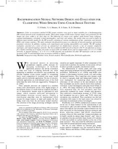
Fig. 3. The incremental learning curve in the case of fourteen rules trined on 20 instances in the promoter domain as the initial knowledge. In contrast to Fig. 2, the neural network would always be adapted to a new instance when the instance was in conflict with the old network knowledge.

TABLE I IRISDOMAIN: TESTOF INCREMENTAL LEARNING CAPABILITY Initial Knowledge

1 instance 1 rule 2 rules 3 rules 4 rules

MLP (15 instances)

lnstanca Index

Fig. 2. The incremental learning curve in the case of fourteen rules trained on 20 instances in the promoter domain as the initial knowledge.

Classification Accuracy initial 33.3% 33.3% 66.0% 93.3% 93.3%

I

best 97.3% 98.7% 96.7% 98.0% 98.7%

94.0% 98.0%

I

final

I 97.3% 97.3% 96.0% 98.0% 98.7% 97.3%

I

2 3

10

4

8 6

3

5

TABLE I1 FRO,MOTER DOMAIN: TESTOF INCREMENTAL LEARNING CAPABILITY Initial Knowledge

Classification Accuracy initial

has four attributes: septal length, septal width, petal length, and petal width. Each attribute of all iris instances was discretized into three levels. Four rules were used as the initial knowledge. Because there are two inconsistent instances due to discretization, the best possible performance in terms of classification accuracy is 98.7%. The second domain was the recognition of promoters in DNA nucleotide strings. There are 53 positive instances and 53 negative instances. Each instance is composed of 57 sequential nucleotides: fifty nucleotides before and six following the site where transcription initiates. Nucleotides have four possible base types: A (Adenine), G (Guanine), C (Cytosine), and T (Thymine). In this domain, we used the 14 rules given in [14]. We evaluated the performance of an incremental learning system in the respects of memorization of old knowledge and generalization to unseen instances. Suppose n instances are available to test our system. We test the network against the n instances when the network is learning the kth instance. The result reflects how well the network remembers k - 1 instances

I

Number of Hidden Units initial final 1 I 9 1 9

14 rules (20 instances) 14 rules (52 instances)

I best I final

Number of Hidden Units initial I final

84.9%

96.2%

96.2%

14

14

95.3%

99.1%

99.1%

14

14

and how well it generalizes to n - k instances. As k approaches n, the test on generalization capability is de-emphasized. Initial knowledge exists in four forms: Initial rules which are directly mapped into a neural network without initial training. Initial rules which are directly mapped into a neural network, which is then trained on a certain number of initial instances. In the Tables I and 11, this case is shown by putting the number of initial instances in parentheses under the number of initial rules. Initial instances used to train a fully connected multilayer perceptron (MLP) before incremental learning starts. An initial single instance which is directly mapped into a neural network without initial training.

Authorized licensed use limited to: Tamkang University. Downloaded on March 15,2010 at 23:24:48 EDT from IEEE Xplore. Restrictions apply.

IEEE TRANSACTIONS ON NEURAL NETWORKS, VOL. 7, NO. 3, MAY 1996

The test results are summarized in Tables 1 and 11. The final performances of the IBPLN are comparable with standard backpropagation learning (nonincremental) in both domains. The learning- curves in all these cases show ”0th convergence with minor fluctuation through the process. See in ~ i 1 ~ 2.~we .also experimented with sample how contradictions between the new data and old network knowledge were handled. The default is that the new data is simply ignored in this circumstmce. Fig. 3 shows the learning curve when the neural network would always be adapted to the new data despite contradiction with previous knowledge, As it appears, learning becomes less smooth in this case.

V. CONCLUSION The standard backpropagation network is not an incremental learner by its nature. The network can, however, perform incremental learning if the network repeatedly sees redundant instances. But this strategy is not useful practically since it requires many instances seen before the network converges. In this paper, we present a new incremental learning method for pattern recognition, the IBPLN, which employs bounded weight modification and structural adaptation learning rules and applies initial knowledge to constrain the learning process. The viability of this approach has been demonstrated for classification problems including the iris and the promoter domains. REFERENCES [I] E. B. Baum and D. Haussler, “What size net gives valid generalization?” Neural Computa., vol. 1, pp. 151-160, 1989.

761

[2] G. A. Carpenter, S. Grossberg, N. Markuzon, J. H. Reynolds, and D.B. Rosen, “Fuzzy ARTMAP: A neural-networkarchitecture for incremental supervised learning of analog multidimensional maps,” IEEE Trans. Neural Networks, vol. 3, pp. 698-713, 1992. 131 R. 0. Duda and P. E. Hart. Pattem Classification and Scene Analvsis. New York: Wiley, 1973. [41 S . E. Fahlman and c . Lebiere, “The cascade-correlation learning architecture,” School Comput. Sci., Carnegie Mellon Univ., Pittsburgh, PA, Tech. Rep. CMU-CS-90-100, 1990. 151 L. M. Fu, “Knowledge-based connectionism for revising domain theories,” IEEE Trans. S W . , Man, Cybem., vol. 23, pp. 173-182, 1993. [6l -, Neural Networks in Computer Intelligence. New York: McGraw-Hill. 1994. [7] G. E. Hinton, “Connectionist learning procedures,”Artijicial Intell., vol. 40, pp. 185-234, 1989. [8] P. W. Hollis and J. J. Paulos, “A neural-network learning algorithm tailored for VLSI implementation,” IEEE Trans. Neural Networks, vol. 5, PP. 784-791, 1994. 191 R. -6. Lacher, s. I. Hruska, and D. C. Kuncicky, “Backpropagation learning in expert networks,” IEEE Trans. Neural Networks, vol. 3, pp. 62-72. 1992. [ 101 T. C. Lee, Structure Level Adaptation for ArtiJicial Neural Networks. Boston, MA: Kluwer, 1991. [ l l ] D. C. Park, M. A. El-Sharkawi, and R. J. Marks, 11, “An adaptively trained neural network,” IEEE Trans. Neural Networks, vol. 2, pp. 334-345, 1991. [12] D. E. Rumelhart, G. E. Hinton, and R. J. Williams, “Learning internal representation by error propagation,” in Parallel Distributed Processing: Explorations in the Microstructures of Cognition. Cambridge, MA: MIT Press, 1986, vol. 1. 1131 D. F. Specht, “Probabilistic neural networks and the polynomial adaline as complementary techniques for classification,” IEEE Trans. Neural Networks, vol. 1, pp. 111-121, 1990. [14] G. G. Towell, J. W. Shavlik, and M. 0. Noordewier, “Refinement of approximate domain theories by knowledge-based neural networks,” in Proc. 8th Nat. Con$ ArtiJicialIntell., Boston, MA, 1990, pp. 861-866. [15] Y. Xia and J. Wang, “Neural network for solving linear programming problems with bounded variables,” ZEEE Trans. Neural Networks, vol. 6, pp. 515-519, 1995.

__

Authorized licensed use limited to: Tamkang University. Downloaded on March 15,2010 at 23:24:48 EDT from IEEE Xplore. Restrictions apply.