An Incremental Optimal Weight Learning Machine of Single-Layer

Hindawi Scientific Programming Volume 2018, Article ID 3732120, 7 pages https://doi.org/10.1155/2018/3732120

Research Article An Incremental Optimal Weight Learning Machine of Single-Layer Neural Networks Hai-Feng Ke,1 Cheng-Bo Lu ,2 Xiao-Bo Li,2 Gao-Yan Zhang,1 Ying Mei ,2 and Xue-Wen Shen3 1

School of Computer & Computing Science, Zhejiang University City College, Hangzhou 310015, China College of Engineering, Lishui University, Lishui 323000, China 3 School of Electronics and Information, Zhejiang University of Media and Communications, Hangzhou 310015, China 2

Correspondence should be addressed to Cheng-Bo Lu; [email protected] Received 12 October 2017; Revised 1 January 2018; Accepted 11 January 2018; Published 1 March 2018 Academic Editor: Wenbing Zhao Copyright © 2018 Hai-Feng Ke et al. This is an open access article distributed under the Creative Commons Attribution License, which permits unrestricted use, distribution, and reproduction in any medium, provided the original work is properly cited. An optimal weight learning machine with growth of hidden nodes and incremental learning (OWLM-GHNIL) is given by adding random hidden nodes to single hidden layer feedforward networks (SLFNs) one by one or group by group. During the growth of the networks, input weights and output weights are updated incrementally, which can implement conventional optimal weight learning machine (OWLM) efficiently. The simulation results and statistical tests also demonstrate that the OWLM-GHNIL has better generalization performance than other incremental type algorithms.

1. Introduction Feedforward neural networks (FNNs) have been extensively used in classification applications and regressions [1]. As a specific type of FNNs, single hidden layer feedforward networks with additive models can approximate any target continuous function [2]. Owing to excellent learning capabilities and fault tolerant abilities, SLFNs play an important role in practical applications and have been investigated extensively in both theory and application aspects [3–7]. Maybe the most popular training method for SLFNs classifiers in recent years was gradient-based back-propagation (BP) algorithms [8–12]. BP algorithms can be easily recursively implemented in real time; however, the slow convergence is the bottleneck of BP, where the fast training is essential. In [13], a kind of novel learning machine named extreme learning machine (ELM) is proposed for training SLFNs, where the learning parameters of hidden nodes, including input weights and biases, are randomly assigned and need not be tuned, while output weights can be obtained by simple generalized inverse computation. It has been proven that, even without updating the parameters of the hidden layer, SLFNs with randomly generated hidden neurons and tunable output

weights maintain their universal approximation and excellent generalization performance [14]. It has been shown that ELM is faster than most state-of-the-art training algorithms for SLFNs and it has been applied widely to many practical cases such as classification, regression, clustering, recognition, and relevance ranking problems [15, 16]. Since input weights and hidden layer biases of SLFNs trained with ELM are randomly assigned, the minor changes of data in input vectors maybe cause large changes of data in hidden layer output matrix of the SLFNs. This in turn will lead to large changes of data in the output weight matrix. According to statistical learning theory [17–21], the large changes of data in the output weight matrix will greatly increase both structural and empirical risks of the SLFNs, which will in turn decrease robustness property of the SLFNs regarding the input disturbances. In fact, it has been noted from simulations that the SLFNs trained with the ELM sometimes perform poor generalization performance and robustness with regard to the input disturbances. In view of this situation, OWLM [22] was proposed; it is seen that both input weights and output weights of the SLFNs are globally optimized with the batch learning type of least squares. All feature vectors of classifier can then be placed at the

2

Scientific Programming

prescribed positions in feature space in the sense that the separability of those nonlinearly separable patterns can be maximized, and better generalization performance can be achieved compared with conventional ELM. However, there is still one major issue existing in OWLM, which is OWLM needing more computational cost than ELM, since the input weights are not randomly selected in SLFNs trained with OWLM. With the advent of the big data age, data sets become larger and more complex [23, 24], which reduces the learning efficiency of OWLM further. For implementing OWLM efficiently, this paper proposed an incremental learning machine referred to as optimal weight learning machine with growth of hidden nodes and incremental learning (OWLM-GHNIL). Whenever new nodes are added, the input weights and output weights could be incrementally updated which can implement the conventional OWLM algorithm efficiently. At the same time, owing to the advantages of OWLM, OWLM-GHNIL has better generalization performance than other incremental algorithms such as EM-ELM [25] (an approach that could automatically determine the number of hidden nodes in generalized single hidden layer feedforward networks) and I-ELM [14], which added random hidden nodes to SLFNs only one hidden node each time. The rest of this paper is organized as follows: in Section 2, the OWLM is briefly described. In Section 3, we present OWLM-GHNIL in detail and analyze its computational complexity. Simulation results are then presented in Section 4, showing that our proposed approach performs more efficiently and has better generalization performance than some existing methods. In Section 5, we give conclusion.

w11 y1

x(k)

11

D

O1 (k)

x(k − 1) D

O2 (k)

D Om (k)

x(k − n + 2) D x(k − n + 1)

Nm  wnN 

yN 

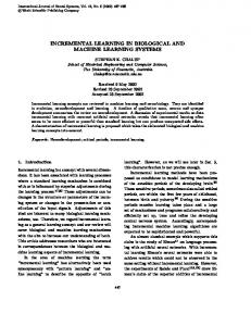
Figure 1: A single hidden layer neural network with linear nodes and an input tapped delay line.

and input weight matrix 𝑊 = [𝑤1 , 𝑤2 , . . . , 𝑤𝑁 ̃] , 𝑤𝑖 = [𝑤𝑖1 , 𝑤𝑖2 , . . . , 𝑤𝑛𝑖 ]

𝑇

and output weight matrix

2. Brief of the Optimal Weight Learning Machine

𝛽 = [𝛽1 , 𝛽2 , . . . , 𝛽𝑚 ] ,

In this section, we briefly describe the OWLM. For 𝑁 given input pattern vectors 𝑥1 (𝑘), 𝑥2 (𝑘), . . ., 𝑥𝑁(𝑘), as well as 𝑁 corresponding desired output data vectors 𝑜1 (𝑘), 𝑜2 (𝑘), . . . , 𝑜𝑁(𝑘),respectively, N linear output equations of SLFNs in Figure 1 can be obtained as 𝐻𝛽 = 𝑂,

(1)

𝛽𝑖 = [𝛽𝑖1 , 𝛽𝑖2 , . . . , 𝛽𝑖𝑁 ̃] .

𝑇

𝐻 = [𝑥1 (𝑘) 𝑥2 (𝑘) ⋅ ⋅ ⋅ 𝑥𝑁 (𝑘)] 𝑊

(5)

Let 𝑦1 , 𝑦2 , . . . , 𝑦𝑁 be 𝑁 feature vectors, corresponding to the input data vectors 𝑥1 , 𝑥2 , . . . , 𝑥𝑁. Then we have [𝑦1 𝑦2 𝑦3 ⋅ ⋅ ⋅ 𝑦𝑁] = 𝑊𝑇 [𝑥1 𝑥2 𝑥3 ⋅ ⋅ ⋅ 𝑥𝑁] ,

(6)

or 𝑌 = 𝑊𝑇 𝑋.

where

(4)

(7)

Let the 𝑁 reference feature vectors be described by

𝑥1 𝑇 𝑤1 𝑥1 𝑇 𝑤2 ⋅ ⋅ ⋅ 𝑥1 𝑇 𝑤𝑁 ̃

[ 𝑇 ] [ 𝑥2 𝑤1 𝑥2 𝑇 𝑤2 ⋅ ⋅ ⋅ 𝑥2 𝑇 𝑤 ̃ ] 𝑁] [ ] =[ [ .. .. .. .. ] = 𝑋𝑊, [ . ] . . . [ ] 𝑇 𝑇 𝑇 ̃] [𝑥𝑁 𝑤1 𝑥𝑁 𝑤2 ⋅ ⋅ ⋅ 𝑥𝑁 𝑤𝑁

𝑌𝑑 = [𝑦𝑑1 𝑦𝑑2 𝑦3𝑑 ⋅ ⋅ ⋅ 𝑦𝑑𝑁] . (2)

with 𝑇

𝑋 = [𝑥1 (𝑘) , 𝑥2 (𝑘) , . . . , 𝑥𝑁 (𝑘)] , 𝑥𝑖 (𝑘) = [𝑥𝑖1 (𝑘) , 𝑥𝑖2 (𝑘) , . . . , 𝑥𝑖𝑛 (𝑘)]

(8)

(3)

Generally, as described in [22], the selection of the 𝑁 desired feature vectors in (8) mainly depends on the characteristics of the input vectors. By optimizing the input weights of the SLFNs in Figure 1, the OWLM can place the feature vectors of the SLFNs at the “desired position” in feature space. The purpose of the assignment is to further maximize the separability of the vectors in the feature space so that the generalization performance and robustness, seen from the output layer of the SLFNs, can be greatly improved, compared with the SLFNs trained with ELM.

Scientific Programming

3

The design of the optimal input weight of the SLFNs can be formulated by the following optimization problem: 1 󵄩 󵄩2 𝜆 { 󵄩󵄩󵄩󵄩𝜀𝑓 󵄩󵄩󵄩󵄩 + 1 ‖𝑊‖2 } 2 2

Minimize

(9)

𝑇

subject to 𝜀𝑓 = 𝑌𝑑 − 𝑌 = 𝑌𝑑 − 𝑊 𝑋, where 𝜆 1 is a positive real regularization parameter. The optimal input weight matrix was derived as follows: 𝑇 −1

𝑇

𝑊 = (𝜆 1 𝐼 + 𝑋𝑋 ) 𝑋𝑌𝑑 .

𝜆 󵄩 󵄩2 1 { ‖𝜀‖2 + 2 󵄩󵄩󵄩𝛽󵄩󵄩󵄩 } 2 2

(11)

subject to 𝜀 = 𝑂 − 𝑇 = 𝐻𝛽 − 𝑇,

−1

−1

𝑊0 = (𝑋𝑋𝑇 + 𝜆 1 𝐼) 𝑋𝑌𝑑0 𝑇 ,

(13)

𝐻0 = 𝑋𝑇 𝑊0

(14) −1

𝛽0 = (𝐻0 𝑇 𝐻0 + 𝜆 2 𝐼) 𝐻0 𝑇 𝑇,

(12)

(15)

where 𝑌𝑑0 is an 𝑚 × 𝑁 matrix consisting of 𝑁 desired feature vectors. Let 𝐸(𝐻𝑖 ) = min‖𝐻𝑖 𝛽𝑖 − 𝑇‖ be the network output error; if 𝐸(𝐻0 ) is less than the target error 𝜀 > 0, then no new hidden nodes need to be added and the learning procedure completes. Otherwise, we could add 𝑛 new nodes to the existing SLFNs; then 𝑌𝑑0 𝑊1 = (𝑋𝑋 + 𝜆 1 𝐼) 𝑋 [ ] 𝑌𝑑1 −1

𝑇

where 𝜆 2 is a positive real regularization parameter. The optimal output weight matrix was derived as follows: 𝛽 = (𝜆 2 𝐼 + 𝐻𝑇 𝐻) 𝐻𝑇 𝑇.

Given SLFNs with initial hidden nodes 𝑚 and a training set {(𝑥𝑖 , 𝑡𝑖 )}𝑁 𝑖=1 let 𝑁 be the number of input patterns, let 𝑙 be the length of the input patterns, and let ℎ be the length of the output patterns. We have

(10)

Similarly, to minimize the error between the desired output pattern 𝑇 and the actual output pattern 𝑂, the design of the optimal output weight of the SLFNs can be formulated by the following optimization problem: Minimize

3. Growing Hidden Nodes and Incrementally Updating Weights

𝑇

(16)

−1

= [𝑊0 (𝑋𝑋𝑇 + 𝜆 1 𝐼) 𝑋𝑌𝑑1 𝑇 ] = [𝑊0 Δ𝑊0 ] , where 𝑌𝑑1 is an 𝑛 × 𝑁 matrix consisting of 𝑁 desired feature vectors. Then,

The optimal weight learning machine [22] can be summarized as follows.

𝐻1 = 𝑋𝑇 [𝑊0 Δ𝑊0 ] = [𝐻0 𝑋𝑇 Δ𝑊0 ] = [𝐻0 , Δ𝐻0 ] ,

Algorithm OWLM. Given a training set {(𝑥𝑖 , 𝑡𝑖 )}𝑁 𝑖=1 , as well as ̃ hidden node number 𝑁, do the following steps.

𝛽1 = ([𝐻0 , Δ𝐻0 ] [𝐻0 , Δ𝐻0 ] + 𝜆 2 𝐼) [𝐻0 , Δ𝐻0 ] 𝑇

Step 1. Randomly assign hidden node parameters (𝑤𝑖 , 𝑏𝑖 ), 𝑖 = ̃ 1, . . . , 𝑁. Step 2. Calculate the hidden layer output matrix 𝐻 by (2).

Step 4. Recalculate the hidden layer output matrix 𝐻new by 𝑊new . Step 5. Calculate the output weight matrix 𝛽 by (12). Obviously, the OWLM needs more training time compared with ELM, since it needs additional computational cost for computing the input weight matrix. 𝐻0 𝑇 Δ𝐻0

Δ𝐻0 𝑇 𝐻0

Δ𝐻0 𝑇 Δ𝐻0 + 𝜆 2 𝐼 −1

=(

−1

𝐻0 𝑇 Δ𝐻0

) + 𝜆 2 𝐼) = (( Δ𝐻0 𝑇 𝐻0 Δ𝐻0 𝑇 Δ𝐻0 𝑇

(17)

⋅ [𝐻0 , Δ𝐻0 ] 𝑇 −1

𝐻0 𝑇 𝑇 ⋅( ). Δ𝐻0 𝑇 𝑇 The Schur complement 𝑃(𝑃 = (Δ𝐻0 𝑇 Δ𝐻0 + 𝜆 2 𝐼) − Δ𝐻0 𝑇 𝐻0 (𝐻0 𝑇 𝐻0 + 𝜆 2 𝐼)−1 𝐻0 𝑇 Δ𝐻0 ) of 𝐻0 𝑇 𝐻0 + 𝜆 2 𝐼 is invertible by choosing the suitable 𝜆 2 . Then, using the result on the inversion of 2 × 2 block matrices [26], we can get

−1

𝐻0 𝑇 𝐻0 + 𝜆 2 𝐼 (𝐻0 𝑇 𝐻0 + 𝜆 2 𝐼)

𝐻0 𝑇 𝐻0

𝑇

𝐻0 𝑇 Δ𝐻0 𝐻0 𝑇 𝐻0 + 𝜆 2 𝐼 ) =( Δ𝐻0 𝑇 𝐻0 Δ𝐻0 𝑇 Δ𝐻0 + 𝜆 2 𝐼

Step 3. Calculate the input weight matrix 𝑊new by (10).

(

−1

𝑇

) −1

−1

+ (𝐻0 𝑇 𝐻0 + 𝜆 2 𝐼) (𝐻0 𝑇 Δ𝐻0 ) 𝑃−1 (Δ𝐻0 𝑇 𝐻0 ) (𝐻0 𝑇 𝐻0 + 𝜆 2 𝐼) −1

−𝑃−1 (Δ𝐻0 𝑇 𝐻0 ) (𝐻0 𝑇 𝐻0 + 𝜆 2 𝐼)

(18)

−1

− (𝐻0 𝑇 𝐻0 + 𝜆 2 𝐼) (𝐻0 𝑇 Δ𝐻0 ) 𝑃−1 𝑃−1

);

4

Scientific Programming

then −1

𝐻0 𝑇 Δ𝐻0 𝐻0 𝑇 𝐻0 + 𝜆 2 𝐼 𝐻0 𝑇 𝛽1 = ( ( )𝑇 ) Δ𝐻0 𝑇 𝐻0 Δ𝐻0 𝑇 Δ𝐻0 + 𝜆 2 𝐼 Δ𝐻0 𝑇 −1

=(

−1

−1

−1

=(

−1

(𝐻0 𝑇 𝐻0 + 𝜆 2 𝐼) 𝐻0 𝑇 𝑇 + (𝐻0 𝑇 𝐻0 + 𝜆 2 𝐼) (𝐻0 𝑇 Δ𝐻0 ) 𝑃−1 (Δ𝐻0 𝑇 𝐻0 ) (𝐻0 𝑇 𝐻0 + 𝜆 2 𝐼) 𝐻0 𝑇 𝑇 − (𝐻0 𝑇 𝐻0 + 𝜆 2 𝐼) (𝐻0 𝑇 Δ𝐻0 ) 𝑃−1 Δ𝐻0 𝑇 𝑇 ) −1 −𝑃−1 (Δ𝐻0 𝑇 𝐻0 ) (𝐻0 𝑇 𝐻0 + 𝜆 2 𝐼) 𝐻0 𝑇 𝑇 + 𝑃−1 Δ𝐻0 𝑇 𝑇

(19)

−1

𝛽0 + 𝑄0 − 𝑅0 𝛽0 + (𝐻0 𝑇 𝐻0 + 𝜆 2 𝐼) (𝐻0 𝑇 Δ𝐻0 ) 𝑃−1 (Δ𝐻0 𝑇 𝐻0 ) 𝛽0 − (𝐻0 𝑇 𝐻0 + 𝜆 2 𝐼) (𝐻0 𝑇 Δ𝐻0 ) 𝑃−1 Δ𝐻0 𝑇 𝑇 )=( ). 𝑇 𝑇 −1 −1 𝑈0 + 𝑉0 −𝑃 (Δ𝐻0 𝐻0 ) 𝛽0 + 𝑃 Δ𝐻0 𝑇

To save computational cost, 𝑄0 , 𝑅0 , 𝑈0 , and 𝑉0 in (19) should be computed as the following sequence: 𝑃−1 (Δ𝐻0 𝑇 𝐻0 ) 󳨀→ 𝑃−1 (Δ𝐻0 𝑇 𝐻0 ) 𝛽0 (= 𝑈0 ) , −1

−1

(𝐻0 𝑇 𝐻0 + 𝜆 2 𝐼) (𝐻0 𝑇 Δ𝐻0 ) 󳨀→ (𝐻0 𝑇 𝐻0 + 𝜆 2 𝐼) ⋅ (𝐻0 𝑇 Δ𝐻0 ) 𝑈0 (= 𝑄0 ) , 𝑃−1 Δ𝐻0 𝑇 󳨀→ 𝑃−1 Δ𝐻0 𝑇 𝑇 (= 𝑉0 )

(20)

−1

󳨀→ (𝐻0 𝑇 𝐻0 + 𝜆 2 𝐼) (𝐻0 𝑇 Δ𝐻0 ) ⋅ 𝑃−1 Δ𝐻0 𝑇 𝑇 (= 𝑅0 ) . Given the number of initial hidden nodes 𝑚0 , the maximum number of hidden nodes 𝑚max , and the expected output error 𝜀, the OWLM-GHNIL for the SLFNs with the mechanism of growing hidden nodes can be summarized as the following two steps. Algorithm OWLM-GHNIL Step 1 (initialization step). (1) Compute 𝑊0 , 𝐻0 , 𝛽0 by (13)–(15). (2) Compute the corresponding output error 𝐸(𝐻0 ) = min ‖𝐻0 𝛽0 − 𝑇‖. Step 2 (recursively incremental step). Let 𝑘 = 0, and while 𝑚𝑘 < 𝑚max and 𝐸(𝐻𝑘 ) > 𝜀, (1) 𝑘 = 𝑘 + 1;

Moreover, the convergence of the OWLM-GHNIL can be guaranteed by the Convergence Theorem in [25]. Now, we begin to analyze computational complexity of the updated work. The computational complexity, which we consider, expresses the total number of required scalar multiplications. Some matrix computations need not be done repeatedly including the inversion of matrix in (13), since they have been obtained in the process of computing 𝑊𝑘 , 𝐻𝑘 , 𝛽𝑘 . Then it requires 𝑙𝑁𝑛, 𝑙𝑁𝑛, and 2𝑚𝑘 𝑛2 + 𝑚𝑘 𝑛𝑁 + 3𝑚𝑘 𝑛ℎ + 2𝑚𝑘 2 𝑛 + 2𝑛2 𝑁 + 𝑛𝑁ℎ + 𝑛3 multiplications for 𝑊𝑘+1 , 𝐻𝑘+1 , and 𝛽𝑘+1 , respectively. Thus, the total computational complexity for the weights 𝑊𝑘+1 and 𝛽𝑘+1 is 𝐶OWLM-GHNIL = 2𝑙𝑁𝑛 + 2𝑚𝑘 𝑛2 + 𝑚𝑘 𝑛𝑁 + 3𝑚𝑘 𝑛ℎ + 2𝑚𝑘 2 𝑛 + 2𝑛2 𝑁 + 𝑛𝑁ℎ + 𝑛3 .

(21)

If we compute 𝑊𝑘+1 and 𝛽𝑘+1 by (10) and (12) directly, it will cost 𝐶OWLM = 𝑙3 + 2𝑙2 𝑁 + 2𝑙𝑁(𝑚𝑘 + 𝑛) + 2(𝑚𝑘 + 𝑛)2 𝑁 + (𝑚𝑘 + 𝑛)3 + (𝑚𝑘 + 𝑛)𝑁ℎ multiplications. Since in most applications 𝑚𝑘 and 𝑛 can be much smaller than the number of training samples N: 𝑚𝑘 , 𝑛 ≪ 𝑁 and h and l are often small number in practical applications, then, with the growth of 𝑚𝑘 , n, 𝐶OWLM

𝐶OWLM-GHNIL

2

≈

2 (𝑚𝑘 + 𝑛) ; 𝑚𝑘 𝑛 + 2𝑛2

(22)

when 𝑛 = (1/2)𝑚𝑘 , 𝐶OWLM

≈ 4.5;

(23)

𝐶OWLM ≈ 8.3. 𝐶OWLM-GHNIL

(24)

𝐶OWLM-GHNIL

(2) randomly add 𝑛 (𝑛 need not be kept constant) hidden nodes to the existing network; then 𝑊𝑘+1 , 𝐻𝑘+1 , 𝛽𝑘+1 can be calculated by (16)–(19).

when 𝑛 = (1/4)𝑚𝑘 ,

End

It can be seen that the OWLM-GHNIL is much more efficient than the conventional OWLM in such cases. Similarly, we can get the computational complexity of the EM-ELM and ELM, respectively.

Different from conventional OWLM which needs recalculating the input weight matrix and output weight matrix, whenever the network architecture is changed, the OWLMGHNIL only needs updating the input weight matrix and output weight matrix incrementally each time; that is why it can reduce the computational complexity significantly.

𝐶EM-ELM = 𝑙𝑁𝑛 + 2𝑚𝑘 𝑛2 + 𝑚𝑘 𝑛𝑁 + 3𝑚𝑘 𝑛ℎ + 2𝑚𝑘 2 𝑛 + 2𝑛2 𝑁 + 𝑛𝑁ℎ + 𝑛3 ,

Scientific Programming

5 2

3

𝐶ELM = 𝑙𝑁 (𝑚𝑘 + 𝑛) + 2 (𝑚𝑘 + 𝑛) 𝑁 + (𝑚𝑘 + 𝑛)

0.18

(25) Then, we have 𝐶OWLM-GHNIL − 𝐶EM-ELM = 𝑙𝑁𝑛, 𝐶OWLM -𝐶ELM = 𝑙3 + 2𝑙2 𝑁 + 𝑙𝑁 (𝑚𝑘 + 𝑛) .

(26)

Obviously, the difference on computational complexity between OWLM-GHNIL and EM-ELM is much less than the difference between OWLM and ELM.

Average testing accuracy (RMSE)

0.16

+ (𝑚𝑘 + 𝑛) 𝑁ℎ.

0.14 0.12 0.1 0.08 0.06 0.04 0.02 0

4. Simulation Results

sin 𝑥 { , 𝑥 ≠ 0 𝑦 (𝑥) = { 𝑥 𝑥 = 0. {1,

(27)

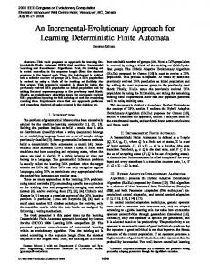
A training set and testing set with 5000 samples, respectively, are generated from the interval (−10, 10) with random noise distributed in [−0.2, 0.2], while testing data remain noise-free. The performances of each algorithm are shown in Figures 2 and 3. In this case, initial SLFNs are given five hidden nodes and then one new hidden node will be added each step until 30 hidden nodes arrive. It can be seen from Figure 2 that the OWLM and the OWLM-GHNIL obtain similar lower testing root mean square error (RMSE) than the EM-ELM in most cases. Figure 3 shows the training time comparison of the three methods in SinC case. We can see that, with the growth of hidden nodes, the OWLM-GHNIL spent similar training time with the EM-ELM but much less than the OWLM in the case of the same number of nodes. In the following, nine real benchmark problems including five regression applications and four classification applications are used for further comparison; all of them are available on the Web. For each case, the training data set and testing data set are randomly generated from its whole data set before each trial of simulation, and average results are obtained over 30 trials for all cases. The features of the benchmark data sets are summarized in Table 1. The generalization performance comparison between the OWLM-GHNIL and two other popular incremental

10

15 20 Number of hidden nodes

25

30

OWLM OWLM-GHNIL EM-ELM

Figure 2: Average testing RMSE of different algorithms in SinC case. 0.1 0.09 0.08 Average training time (s)

In our experiments, all the algorithms are run in such computer environment: (1) operating system: Windows 7 Enterprise; (2) 3.8 GHZ CPU, Intel i5-3570; (3) memory: 8 GB; (4) simulating software: Matlab R2013a. The performance of the OWLM-GHNIL has been compared with other growing algorithms including the EM-ELM, I-ELM, and the conventional OWLM. In order to investigate the performance of the proposed OWLM-GHNIL, some benchmark problems are presented in this section. The OWLM-GHNIL, EM-ELM, and OWLM have first been run to approximate the artificial “SinC” function which is a popular choice to illustrate neural network.

5

0.07 0.06 0.05 0.04 0.03 0.02 0.01 0

5

10

15 20 Number of hidden nodes

25

30

OWLM OWLM-GHNIL EM-ELM

Figure 3: Computational complexity comparison of different algorithms in Sinc case.

ELM-type algorithms, EM-ELM and I-ELM, on regression and classification cases is given in Tables 2 and 3. In the implementation of the EM-ELM and OWLM-GHNIL, initial SLFNs are given 50 hidden nodes and then 25 new hidden nodes will be added each step until 150 hidden nodes arrive. In the case of the I-ELM, the initial SLFNs are given 1 hidden node and then the hidden nodes are added one by one until 150 hidden nodes. As observed from test results of average RMSE and accuracy in Tables 2 and 3, it looks that the OWLM-GHNIL obtained better generalization performance than the EM-ELM and I-ELM. In order to obtain an objective statistical measure, we apply a Student’s 𝑡-test to each data to check if the differences between the OWLM-GHNIL and

6

Scientific Programming Table 1: Details of the data sets used for regression and classification.

Data sets Delta Ailerons Delta Elevators California Housing Computer activity Bank domains COLL20 G50C USPST(B) Satimage

Classes — — — — — 20 2 2 6

Attributes 6 6 8 8 8 1024 50 256 36

Types Regression Regression Regression Regression Regression Classification Classification Classification Classification

# of pieces of training data 3000 4517 8000 4000 4500 1080 414 1509 3217

# of pieces of testing data 4129 5000 12,460 4192 3692 360 136 498 3218

Table 2: Comparison of average testing RMSE/accuracy and Student’s 𝑡-test for the data sets between OWLM-GHNIL and EM-ELM. Data sets Delta Ailerons Delta Elevators California Housing Computer activity Bank domains COLL20 G50C USPST(B) Satimage

OWLM-GHNIL RMSE/accuracy 0.0583 0.0896 0.1841 0.0467 0.0212 91.25% 85.31% 90.45% 88.15%

Std. 0.0058 0.0063 0.0032 0.0021 0.0043 0.0332 0.0553 0.0158 0.0368

EM-ELM RMSE/accuracy 0.1023 0.1423 0.2321 0.0392 0.0611 86.33% 87.23% 85.21% 85.37%

Std. 0.0081 0.0154 0.0045 0.0018 0.0032 0.0537 0.0463 0.0547 0.0446

𝑡-Test 𝑝 value 0.003627 0.025436 0.000048 0.628794 0.007694 0.000000 0.065632 0.000000 0.007625

Table 3: Comparison of average testing RMSE/accuracy and Student’s 𝑡-test for the data sets between OWLM-GHNIL and I-ELM. Data sets Delta Ailerons Delta Elevators California Housing Computer activity Bank domains COLL20 G50C USPST(B) Satimage

OWLM-GHNIL RMSE/accuracy 0.0583 0.0896 0.1841 0.0467 0.0212 91.25% 85.31% 90.45% 88.15%

Std. 0.0058 0.0063 0.0032 0.0021 0.0043 0.0332 0.0553 0.0158 0.0368

the other two algorithms are statistically significant (𝑝 value = 0.05, i.e., confidence of 95%). It was shown in Table 2 that, in four of the regression data sets (Delta Ailerons, Delta Elevators, California Housing, and Bank domains) and three of the classification data sets (COLL20, USPST(B), and Satimage), the 𝑡-test gave a significant difference between OWLMGHNIL and EM-ELM with superior generalization performance of the OWLM-GHNIL, whereas no significant difference was found in the two other data sets (computer activity and G50C). In Table 3, the 𝑡-test results show that there was a significant difference between OWLM-GHNIL and I-ELM with superior generalization performance of the OWLMGHNIL in all data sets except computer activity data set.

I-ELM RMSE/accuracy 0.1364 0.2265 0.4365 0.0733 0.1128 78.04% 76.45% 84.33% 80.33%

Std. 0.0223 0.0196 0.0223 0.0072 0.0341 0.0663 0.0772 0.0472 0.0682

𝑡-Test 𝑝-value 0.000493 0.003743 0.000000 0.065475 0.000000 0.000000 0.000482 0.000000 0.001356

5. Conclusion In this paper, we have developed an efficient method, OWLM-GHNIL; it can grow hidden nodes one by one or group by group in SLFNs. The analysis of computational complexity and simulation results on an artificial problem shows that OWLM-GHNIL can significantly reduce the computational complexity of OWLM. The simulation results on nine real benchmark problems including five regression applications and four classification applications also show that OWLM-GHNIL has better generalization performance than the two other incremental algorithms EM-ELM and I-ELM. 𝑡-test gave a significant difference with superior generalization performance of the OWLM-GHNIL further.

Scientific Programming

7

Conflicts of Interest The authors declare that there are no conflicts of interest regarding the publication of this paper.

[15]

Acknowledgments

[16]

This research was supported by Zhejiang Provincial Natural Science Foundation of China under Grant no. LY18F030003, Foundation of High-Level Talents in Lishui City under Grant no. 2017RC01, Scientific Research Foundation of Zhejiang Provincial Education Department under Grant no. Y201432787, and the National Natural Science Foundation of China under Grant no. 61373057.

[17]

[18]

[19]

References [1] C. M. Bishop, Neural Networks for Pattern Recognition, Oxford University Press, New York, NY, USA, 1995. [2] G.-B. Huang and H. A. Babri, “Upper bounds on the number of hidden neurons in feedforward networks with arbitrary bounded nonlinear activation functions,” IEEE Transactions on Neural Networks and Learning Systems, vol. 9, no. 1, pp. 224–229, 1998. [3] X.-F. Hu, Z. Zhao, S. Wang, F.-L. Wang, D.-K. He, and S.-K. Wu, “Multi-stage extreme learning machine for fault diagnosis on hydraulic tube tester,” Neural Computing and Applications, vol. 17, no. 4, pp. 399–403, 2008. [4] T.-Y. Kwok and D.-Y. Yeung, “Objective functions for training new hidden units in constructive neural networks,” IEEE Transactions on Neural Networks and Learning Systems, vol. 8, no. 5, pp. 1131–1148, 1997. [5] E. J. Teoh, K. C. Tan, and C. Xiang, “Estimating the number of hidden neurons in a feedforward network using the singular value decomposition,” IEEE Transactions on Neural Networks and Learning Systems, vol. 17, no. 6, pp. 1623–1629, 2006. [6] X. Luo, J. Deng, W. Wang, J.-H. Wang, and W. Zhao, “A quantized kernel learning algorithm using a minimum kernel risk-sensitive loss criterion and bilateral gradient technique,” Entropy, vol. 19, no. 7, article no. 365, 2017. [7] Y. Xu, X. Luo, W. Wang, and W. Zhao, “Efficient DV-HOP localization forwireless cyber-physical social sensing system: A correntropy-based neural network learning scheme,” Sensors, vol. 17, no. 1, article no. 135, 2017. [8] S. Haykin, Neural networks and learning machines, Pearson, Prentice-Hall, New Jersey, USA, 3rd edition, 2009. [9] S. Kumar, Neural Networks, McGraw-Hill Companies Inc., Columbus, OH, USA, 2006. [10] X. Yao, “Evolving artificial neural networks,” Proceedings of the IEEE, vol. 87, no. 9, pp. 1423–1447, 1999. [11] G. P. Zhang, “Neural networks for classification: a survey,” IEEE Transactions on Systems, Man, and Cybernetics, Part C: Applications and Reviews, vol. 30, no. 4, pp. 451–462, 2000. [12] J. Hertz, A. Krogh, and R. G. Palmer, Introduction to the Theory of Neural Computation, Addison-Wesley Publishing Company, Boston, Mass, USA, 1991. [13] G. B. Huang, Q. Y. Zhu, and C. K. Siew, “Extreme learning machine: theory and applications,” Neurocomputing, vol. 70, no. 1–3, pp. 489–501, 2006. [14] G. Huang, L. Chen, and C. Siew, “Universal approximation using incremental constructive feedforward networks with

[20] [21]

[22]

[23]

[24]

[25]

[26]

random hidden nodes,” IEEE Transactions on Neural Networks and Learning Systems, vol. 17, no. 4, pp. 879–892, 2006. S.-F. Ding, X.-Z. Xu, and R. Nie, “Extreme learning machine and its applications,” Neural Computing and Applications, vol. 25, no. 3, pp. 549–556, 2014. X. Luo, Y. Xu, W. Wang et al., “Towards enhancing stacked extreme learning machine with sparse autoencoder by correntropy,” Journal of The Franklin Institute, 2017. M. Anthony and P. L. Bartlett, Neural Network Learning: Theoretical Foundations, Cambridge University Press, Cambridge, UK, 1999. V. N. Vapnik, Statistical Learning Theory, Adaptive and Learning Systems for Signal Processing, Communications, and Control, Wiley- Interscience, New York, NY, USA, 1998. L. Devroye, L. Gy¨orfi, and G. Lugosi, A Probabilistic Theory of Pattern Recognition, vol. 31 of Stochastic Modelling and Applied Probability, Springer-Verlag New York, Berlin, Germany, 1996. R. O. Duda, P. E. Hart, and D. G. Stork, Pattern Classification, Wiley-Interscience, New York, NY, USA, 2nd edition, 2001. L. Breiman, J. H. Friedman, R. A. Olshen, and C. J. Stone, Classification and Regression Trees, Wadsworth, Belmont, Mass, USA, 1984. Z. Man, K. Lee, D. Wang, Z. Cao, and S. Khoo, “An optimal weight learning machine for handwritten digit image recognition,” Signal Processing, vol. 93, no. 6, pp. 1624–1638, 2013. X. Luo, J. Deng, J. Liu, W. Wang, X. Ban, and J. Wang, “A quantized kernel least mean square scheme with entropy-guided learning for intelligent data analysis,” China Communications, vol. 14, no. 7, pp. 127–136, 2017. W. Zhao, R. Lun, C. Gordon et al., “A human-centered activity tracking system: toward a healthier workplace,” IEEE Transactions on Human-Machine Systems, vol. 47, no. 3, pp. 343–355, 2017. G. Feng, G.-B. Huang, Q. Lin, and R. Gay, “Error minimized extreme learning machine with growth of hidden nodes and incremental learning,” IEEE Transactions on Neural Networks and Learning Systems, vol. 20, no. 8, pp. 1352–1357, 2009. G. H. Golub and C. F. van Loan, Matrix Computations, The Johns Hopkins University Press, Baltimore, Md, USA, 3rd edition, 1996.

Journal of

Advances in

Industrial Engineering

Multimedia

Hindawi Publishing Corporation http://www.hindawi.com

The Scientific World Journal Volume 2014

Hindawi Publishing Corporation http://www.hindawi.com

Volume 2014

Applied Computational Intelligence and Soft Computing

International Journal of

Distributed Sensor Networks Hindawi Publishing Corporation http://www.hindawi.com

Volume 2014

Hindawi Publishing Corporation http://www.hindawi.com

Volume 2014

Hindawi Publishing Corporation http://www.hindawi.com

Volume 201

Advances in

Fuzzy Systems Modelling & Simulation in Engineering Hindawi Publishing Corporation http://www.hindawi.com

Hindawi Publishing Corporation http://www.hindawi.com

Volume 2014

Volume 2014

Submit your manuscripts at https://www.hindawi.com

-RXUQDORI

&RPSXWHU1HWZRUNV DQG&RPPXQLFDWLRQV

 Advances in 

Artificial Intelligence +LQGDZL3XEOLVKLQJ&RUSRUDWLRQ KWWSZZZKLQGDZLFRP

Hindawi Publishing Corporation http://www.hindawi.com

9ROXPH

International Journal of

Biomedical Imaging

Volume 2014

Advances in

$UWLÀFLDO 1HXUDO6\VWHPV

International Journal of

Computer Engineering

Computer Games Technology

Hindawi Publishing Corporation http://www.hindawi.com

Hindawi Publishing Corporation http://www.hindawi.com

Advances in

Volume 2014

Advances in

Software Engineering Volume 2014

Hindawi Publishing Corporation http://www.hindawi.com

Volume 2014

Hindawi Publishing Corporation http://www.hindawi.com

Volume 201

Hindawi Publishing Corporation http://www.hindawi.com

Volume 2014

International Journal of

Reconfigurable Computing

Robotics Hindawi Publishing Corporation http://www.hindawi.com

Computational Intelligence and Neuroscience

Advances in

Human-Computer Interaction

Journal of

Volume 2014

Hindawi Publishing Corporation http://www.hindawi.com

Volume 2014

Hindawi Publishing Corporation http://www.hindawi.com

Journal of

Electrical and Computer Engineering Volume 2014

Hindawi Publishing Corporation http://www.hindawi.com

Volume 2014

Hindawi Publishing Corporation http://www.hindawi.com

Volume 2014