IATSS ReSeARch Vol.32 No.2, 2008 95 ... capacities. maximizing the total trips by private and public travel modes allows policy makers to ..... 4. 3. 2. 1. 0. (15) where, ui. : car ownership of zone i; u0i. : maximum number of car owned at zone i;.
AN INTEGRATED MODELING FRAMEWORK FOR ENVIRONMENTALLY EFFICIENT CAR OWNERSHIP AND TRIP BALANCE T. FENG, J. ZHANG, A. FUJIWARA
AN INTEGRATED MODELING FRAMEWORK FOR ENVIRONMENTALLY EFFICIENT CAR OWNERSHIP AND TRIP BALANCE Tao FENG
Junyi ZHANG
Akimasa FUJIWARA
Ph.D Candidate Graduate School for International Development and Cooperation Hiroshima University Hiroshima, Japan
Associate Professor Graduate School for International Development and Cooperation Hiroshima University Hiroshima, Japan
Professor Graduate School for International Development and Cooperation Hiroshima University Hiroshima, Japan
(Received July 15, 2008)
Urban transport emissions generated by automobile trips are greatly responsible for atmospheric pollution in both developed and developing countries. To match the long-term target of sustainable development, it seems to be important to specify the feasible level of car ownership and travel demand from environmental considerations. This research intends to propose an integrated modeling framework for optimal construction of a comprehensive transportation system by taking into consideration environmental constraints. The modeling system is actually a combination of multiple essential models and illustrated by using a bi-level programming approach. In the upper level, the maximization of both total car ownership and total number of trips by private and public travel modes is set as the objective function and as the constraints, the total emission levels at all the zones are set to not exceed the relating environmental capacities. Maximizing the total trips by private and public travel modes allows policy makers to take into account trip balance to meet both the mobility levels required by travelers and the environmentally friendly transportation system goals. The lower level problem is a combined trip distribution and assignment model incorporating traveler’s route choice behavior. A logit-type aggregate modal split model is established to connect the two level problems. In terms of the solution method for the integrated model, a genetic algorithm is applied. A case study is conducted using road network data and person-trip (PT) data collected in Dalian city, China. The analysis results showed that the amount of environmentally efficient car ownership and number of trips by different travel modes could be obtained simultaneously when considering the zonal control of environmental capacity within the framework of the proposed integrated model. The observed car ownership in zones could be increased or decreased towards the macroscopic optimization objective with zonal limit of emissions. Key Words: Car ownership, Integrated model, Environmental capacity, Bi-level programming, Trip balance, Genetic algorithm
1. INTRODUCTION Looking at the progress of transportation development, there always exists the paradox between motorization and its resulting environmental loads. Many existing studies have shown that traffic emissions are increasingly responsible for urban air pollution. For example, in Britain, at least three-quarters of CO, a quarter of CO2 and more than a half of NOx comes from car traffic1. A similar situation has also appeared in most Chinese cities where it is estimated that about 60% of CO, 50% of NOx and 30% of HC are created by car traffic 2. However, considering economic development in developing countries such as China, the increasing desire of car ownership and the resulting increase of car travel demand will continue into the future. Therefore, policies of solving environmental issues caused by such a trend are urged. Among varieties of environmentally friendly poli-
cies, emphasis is often put on setting various limitations on car use rather than its ownership. This might be due to the consideration of negative impacts of car ownership control policies on economic activities, because the automobile industry is becoming a more and more important sector of the economies of developing countries. Another fact is that automobile makers in developed countries have been attracted by the potential market and cheap skillful human resources in developing countries and have started on-site automobile production to meet both domestic and international demand. Actually, the increase of car ownership that is inherently affected by consumers’ preferences is inevitably restricted by various factors such as household income, taxation of car ownership and usage, the available parking space and the level of parking charges, road capacity, and environmental policies. Taking specifically into account the ever increasing environmental impacts of car traffic, its emissions should be controlled IATSS Research Vol.32 No.2, 2008
95
TRANSPORTATION
within certain thresholds, namely environmental capacity (EC), to realize sustainable development. Among most of the available control policies, one of the environmentally friendly alternatives is to persuade people to travel by public travel modes instead of private car. In other words, policies to keep a desirable balance between private and public travel modes (called trip balance in this study) should be promoted. Therefore, it becomes necessary to establish an integrated modeling framework for predicting the feasible extent of mobility level (realized by private and public modes) and acceptable car ownership under the consideration of environmental sustainability. To realize such an idea, one of the crucial issues is to clarify the aforementioned EC. It is generally difficult to give an accurate definition about EC and there is no widely accepted definition either. However, we understand that EC refers to the maximum level of environmental emissions (e.g., NOx, SOx and CO) that a city or a region could accommodate to meet the traveler’s mobility level. There are many factors affecting the level of EC where some can be easily observed (e.g., green space, meteorological conditions, and geography), others may not be observable (e.g., motivation of pro-environmental behavior, and future technological innovation). In reality, standards of air quality in a city are often adopted as the threshold for evaluating the pollution level. Other relating long-term environmental considerations often greatly rely on experts’ experiences, which are sometimes arbitrary and lack theoretical support. Little research has been done related to the EC and in this sense, measuring the EC is still an illsolved problem and needs to be further investigated. Under such circumstances, here, the concept of frontier which has been widely applied for efficiency analysis in the field of econometrics is adopted as a measurement of EC. The EC is defined as the emission frontier by assuming there is no inefficiency in a transportation system. Regarding EC as the only constraint target for traffic emission, this paper attempts to propose an integrated modeling framework, which estimates the maximal mobility level, i.e., the level of environmentally efficient car ownership and the number of trips by both private and public travel modes simultaneously, by explicitly incorporating the influences of transportation network performance and the EC. Here, a bi-level (BL) programming approach is adopted to calculate the integrated model system, where two levels of problems are illustrated by setting different optimization objectives with different decision variables that are interacted with each other. In the upper level, the maximization of both total car ownership and total num-
96
IATSS Research Vol.32 No.2, 2008
ber of trips by private and public travel modes is set as the objective function and as the constraints, the total emission levels at all the zones are set to not exceed the relating environmental capacities (i.e., emission frontier). The lower level problem is a combined trip distribution and assignment model incorporating traveler’s route choice behavior. A logit-type aggregate modal split model is further established to connect the two level problems. The BL programming approach allows for the simultaneous consideration of both bottom-up and top-down policy decision-making and could consequently be more effective to achieve smooth consensus building among different stakeholders, compared with other existing approaches. The proposed modeling approach could be further extended to include more policy objectives and more constraints related to policy implementation at the upper level and to incorporate dynamic elements into the lower level for the sake of short-term travel demand management and long-term planning. For the former extension, a comprehensive set of sustainable development goals should be considered and for the latter extension, a dynamic travel demand modeling system should be included to accommodate both long-term and short-term changes of transportation demand and supply. Since the computation burdens of the proposed integrated modeling approach is very high, as an initial attempt, this study tries to confirm its performance by considering only static elements and a limited set of sustainable development requirements. For such purposes, a case study using the data of Dalian city, China is carried out. The total simulation process is realized based on genetic algorithm. Other parts of this paper are organized as follows. Section 2 gives a literature review, followed by Section 3 that describes the integrated model. A case study based on the person-trip data collected in Dalian City, China is conducted and research findings are discussed in Section 4. Finally the study is concluded with the discussion on future research issues.
2. LITERATURE REVIEW Increase of car ownership was originally thought to be influenced by the economic level (e.g., GDP) and predicted based on the S-curve (logistic) function 3-5. However, such a modeling approach has some shortcomings, one of which is that it does not reflect people’s preferences in the model and consequently cannot be used as a tool to evaluate the relevant policies to control car ownership. To overcome such shortcomings of the economic indicator based model, in recent years, many studies have
AN INTEGRATED MODELING FRAMEWORK FOR ENVIRONMENTALLY EFFICIENT CAR OWNERSHIP AND TRIP BALANCE T. FENG, J. ZHANG, A. FUJIWARA
been conducted to explore other factors that affect car ownership behavior. Among those studies, the disaggregate analysis approach that is based on household or individual preference has been dominating the literature 6-8. The models based on such an approach are usually built on the principle of random utility maximization. Concerning the car-related policies that aim to mitigate negative effects of car traffic (e.g., congestion, accidents and emissions), for example, Mueller and Haan 9 proposed a multi-agent model to simulate purchases of passenger cars under future policies related to fuel consumption, which mainly consist of cash rewards as a bonus and sales tax as malus. In the model, 24 different agent types are used to forecast the responses of individuals under future bonusmalus schemes. Different from these studies, this paper attempts to derive the desirable level of car ownership from environmental considerations of the whole city, rather than from individual preferences. Environmental analyses at the roadside are usually modeled as the problem of emission estimation and pollutant dispersion. Nowadays, various methods have been proposed for either of those discussions. A comprehensive review on different measurement approaches of emission estimation was written by Smit 10. The commonly used approach to observe link-based emission depends mainly on the emission factors which are related to actual traffic conditions such as average vehicle speed 10. Furthermore, Park et al.11 proposed a methodology using a vehicle-mapping table which can convert Vehicle Miles Traveled (VMT) fractions from FHWA types to MOBILE types that utilize readily available data sources. However, to realize such a measure in real cases generally involves high expenditure. Thus, this paper adopts the average speed model based on existing emission factors suggested by Smit 10. Concerning pollutant dispersion, except the widely discussed Gaussian plume model 12, a series of line source models (e.g., HIWAY, CALINE, GM, and CAL3QHC) have been further developed to improve the prediction accuracy. However, it is still not satisfactorily sufficient to explain pollutant concentrations based on traffic flow characteristics exclusively. Based on this point, artificial intelligent techniques in simulating complex phenomena have received great attention in the literature. Many studies have applied the neural network based model to predict different pollutant concentrations 13-17. The neural network based prediction model increases the model accuracy, but they still inherently depend on the result of emission estimation. Therefore, the environmental problem discussed in this study refers to the effect of traffic
emission. Due to the complexities of environmental systems, environmental capacity is generally defined in qualitatively rather than quantitatively. The Kyoto Protocol requires that the emitted pollutants of six kinds of greenhouse gases from all developed countries in 2012 should be reduced by 5.2% compared with the emission levels in 1990. Most recently, regarding the first pillar of the EU’s strategy, in 2003, the average specific CO2 emission of the fleets are 163 g/km for ACEA (European manufacturers), 172 g/km for JAMA and 179 g/km for KAMA (Japanese and Korean manufacturers) 9. All these regulated values provide a meaningful upper limit for the environmental capacity operationally. However, the problem is how to build a feasible and theoretical formula to calculate the environmental capacity that could be linked with policy instruments. Understanding capacity definition could be two folds; one is the ‘strict limit’ which does not permit any excess for protecting the current system function. In this case, if the threshold value is exceeded, the system is assumed to be destroyed. The second is named the ‘accessible capacity’, which is not the maximum concept but can ensure the system runs efficiently and continuously. This idea is based to some extent on some part of recovery capability of the meteorological system. Actually, if we look at the implication of the later capacity concept from a systematic view, it could be substituted by the frontier environment level when the transportation system operates in its most efficient state. In this case, the capacity analysis could be equivalent to the environment efficiency analysis of the transportation system. Therefore the environmental frontier of the transportation system can be defined as the best environmental condition (the least environmental pollution) under current transportation supplies. The methods for system efficiency analysis have been widely applied in various studies18-20. These days, one can observe an increasing number of studies dealing with efficiency analysis in transportation research. Costa and Markellos 21 evaluated the efficiency of public transport systems during the period 1970 to 1994. Pels et al.22 analyzed the inefficiencies and scale economies of European airport operations. In line with this research stream, this paper makes use of the stochastic frontier analysis (SFA) approach, which can be used to reflect the influence of random shock on the calculation of efficiency. Hereafter, the frontier environmental level calculated from the SFA is used as a measure of the environmental capacity (EC). To derive the desirable level of car ownership from the environmental consideration of the whole city, transIATSS Research Vol.32 No.2, 2008
97
TRANSPORTATION
portation systems are required to be optimized. Such optimization should simultaneously incorporate the current states and the future desirable states of transportation systems. For this purpose, a bi-level (BL) modeling approach has been mostly discussed and examined in a wide range. The BL approach was proposed from the desire to deal with planning goals at an upper level and to represent users’ response behavior to different policies at a lower level. For example, Yang and Yagar 23 resolved the traffic assignment and signal control problems in saturated road networks. In their research, the lower-level problem represents a fixed demand user equilibrium assignment model involving queuing and congestion while the upper-level is an optimization problem about signal control, taking account of drivers’ route choice behavior in response to signal split changes. Gao and Sun 24 presented transit equilibrium network design problems, in which the upper level is a normal transit network design problem, which minimizes total system impendence and total expenses caused by frequency settings, and the lower level is a trip equilibrium assignment model, which present users’ route choice behavior. In addition, Yang25 predicted the O-D demand with the BL optimization models. Tam and Lam26 measured the relationship between road capacity and car ownership, in which the upper level is a maximal car ownership model and the lower level is an equilibrium trip distribution/assignment problem. Moreover, Tam and Lam27, from the view of both travel demand and road network supply, presented the concept of equilibrium of car ownership and gave some empirical analysis taking Hong Kong as an example. Concerning the algorithm of BL programming, a set of approaches have been proposed such as a sensitivity analysis based algorithm23,26, simulated annealing approach 28, and genetic algorithm29, 30. Bi-level programming is inherently a non-convex problem which is verified to be difficult to find the optimal solution in spite of two linear problems31. Because of the complexity of heuristic algorithms in their application, algorithms based on intelligent techniques have been efficiently applied. Yin29 deduced the genetic algorithm (GA) based approach for bi-level transportation models, and compared the performance of GA with that of the sensitivity based analysis (SBA) algorithm using two numerical studies. The result suggested that GA can reserve similar results with respect to the SBA algorithm but better performance than SBA. Lee et al.30 applied the GA to an equity-based land-use transportation problem which is built with bi-level modeling approach. The GA with penalty functional index is proposed for the constrained optimization problem. This
98
IATSS Research Vol.32 No.2, 2008
paper adopts the concept of GA and designs the modeling process for this bi-level problem. Based on the above literature review, there are several original points of the current paper compared with existing studies. First, this study builds a comprehensive modeling framework to simultaneously represent environmentally efficient mobility (here, referring to car ownership) and trip balance using the BL programming approach. The concept of trip balance is used to calculate the desirable shares of private and public travel modes. Second, a quantitative measure of environmental capacity based on the SFA approach is adopted. A frontier estimation of environmental emission depends on factors of car ownership and population density. The consequence is to obtain the potential maximum of car ownership and total trips by different modes under the consideration of environmental capacity.
3. INTEGRATED MODELING FRAMEWORK 3.1 Basic structure The proposed modeling framework is built with a bi-level programming approach which is composed of two levels of problems named the upper level problem (ULP) and lower level problem (LLP) respectively. The ULP is an optimization problem with the objective of maximizing the sum of zonal car ownership and total number of trips by car and non-car modes, while the ULP is a combined trip distribution and assignment model that explicitly incorporates route choice behavior mechanisms. The integrated mathematical model can be expressed as follow: (1) Upper level problem: c c c c Max: λu ∑ ui + λv ∑∑ (φij ⋅ qij + φij ⋅ qij )�
(1)
s.t. Ei (ui ) ≤ E0 i , i ∈ I �
(2)
i∈I
i
j
Ei (ui ) = ∑ ea , Ai ∈ A�
(3)
ea = γ ak × va × l a , a ∈ A, k ∈ K �
(4)
qijc (ui ) = Qij ⋅ Pijc (u i )�
(5)
qijc (ui ) = Qij ⋅ (1 − Pijc (ui ))�
(6)
0 ≤ ui ≤ u0i , i ∈ I
a ∈ Ai
�
(7)
AN INTEGRATED MODELING FRAMEWORK FOR ENVIRONMENTALLY EFFICIENT CAR OWNERSHIP AND TRIP BALANCE T. FENG, J. ZHANG, A. FUJIWARA
(2) Lower level problem: va
c c c Min: ∑ ∫ ca (x ) dx + ξ1 ∑∑ (qij ln qij − qij )�
(8)
s.t. ∑ f h = qijc , i ∈ I , j ∈ J �
(9)
∑ qijc = Oi , i ∈ I �
(10)
= Dj , j ∈ J �
(11)
a
i
0
j
h∈ H
j∈J
∑q
c ij
i∈I
va = ∑ f hδ ah , a ∈ A, h ∈ H �
(12)
fh , q ≥ 0 , h ∈ H, i ∈ I , j ∈ J �
(13)
h ∈H c ij
(3) Model split model: To connect the upper and lower level problems exp(Vijc )
Pijc ( ui ) =
Vijc = b0 + b1⋅1n(tijc ) + b2⋅ ui + b3⋅ indui + b4⋅ commi� (15)
1 + exp(Vijc )
�
(14)
where, ui : car ownership of zone i; u0i : maximum number of car owned at zone i; c q ij : car trip demand between O-D pair (i, j) ; q cij : non-car trip demand between O-D pair (i, j) ; Ei : total traffic emissions at zone i; E0i : emission capacity at zone i; ea : emission on link a; γ ak : emission factor of category k on link a and k indicates travel speed category; va : link volume; la : length of link a; Qij : total trips between O-D pair (i, j); Pcij : probability of choosing car mode from zone i to j; Ca : travel time on link a; fh : traffic flow on path h; Oi : trip production by car at origin zone i; Dj : trip attraction by car at destination j; t cij : travel time by car from zone i to j; x : dispersion parameter for a gravity-type trip distribution model; V cij, V cij : deterministic term of the utility of choosing and not choosing car from zone i to j, respectively indui : dummy variable of land use for industry commi : dummy variable of land use for commerce I, J : the set of zones; A : the set of links; H : the set of paths; K : the set of travel speed;
fk : traffic flow on path k; lu, lv, f cij, f cij : the pre-defined parameters relating to ui and qij; b0, bi : parameters need to be estimated. The objective function in the upper level is the weighted sum of car ownership and total number of trips. Such objective function allows for simultaneous representation of two or more policy goals and is consequently helpful to trade off different policy emphases. Those parameters λu, λv, f cij, f cij provide the means to reflect different weights of policy goals. These goals should be defined based on consensus building among all the stakeholders related to the targeted policies. Larger value f cij could result in more non-car trips and less car trips simultaneously while ensuring the total number of trips reach the maximum. The indicators such as λu and λv can also be used to assign different emphases between car ownership and trips. The environmental emission from each link is calculated as the product of link length, traffic volume and emission factors that depend on the average driving speed on each link. The emission factors are drawn on from existing literature. The emission Ei from each zone equals the sum of emissions from the links that are included in the zone under study. Therefore, the area and spatial location of each zone affect the emission level. For example, the zones within the central business district (CBD) are mostly at the high density of the road network and consequently show high pollution concentrations, although their areas are in small scales, respectively. Conversely, suburban zones are usually at a large scale, but with lower road network densities, and less pollution than those in the CBD zones. It should be noted that car ownership at each zone is additionally restricted within a certain range [0, u0]. Theoretically, this limit could be equal to or larger than the derived maximum car ownership from the above BL programming approach. The introduction of such a limit is due to the use of the GA algorithm that searches for a feasible solution over the whole range. In the case study, we set the u0 by assuming that the rate of car ownership at each zone is equal to the number of residents that is almost impossible in reality. In this sense, the introduction of such a limit is realistic. The advantage is that such a limit could extremely shorten the calculation time. 3.2 Calculation of environmental capacity The constraint condition is that total environmental emissions from each zone (Ei) must not exceed the IATSS Research Vol.32 No.2, 2008
99
TRANSPORTATION
relating environmental capacity (E0i). Calculation of the environmental capacity at the zonal level would be helpful to effectively control the environmental pollution considering the specific characteristics of different areas. However, this is not an easy task because the capacity could be influenced by various factors. The Kyoto Protocol provides a reference at the nation level but lacks a theoretical base. Here, we propose to apply the stochastic frontier analysis (SFA) which has been applied in numerous studies to evaluate system efficiency. The environmental efficiency here indicates the operation efficiency of the transportation system from the viewpoint of environmental load. The system inputs used in SFA are the indicators of transport infrastructure supply while the output is the observed environmental emission. Then the frontier emission calculated by current explanatory variables is regarded as the named capacity, although it is actually not at the maximum but at the most efficient level. The basic idea of efficiency analysis is that a producer (here, refers to a city or zone) expects the minimum inputs required to produce various outputs, or the maximum output producible with various inputs 32. When analyzing transportation environmental efficiency, the pollutant level can be regarded as the production output from the transportation system. The higher the efficiency means the worse the performance of the system. Regardless of the price information, the efficiency analysis model is actually a cost frontier model. The environmental capacity at the zone or city level will be calculated from the frontier output by use of the validated formula. The well-known Cobb-Douglas formulation for measuring system efficiency is shown as follows:
ln yi = θ 0 +
∑θ
m
ln xim + ε i�
(16)
m∈ M
ε i = ωi + μ i�
(17)
where, yi : total amount of car emissions at city or zone i xim : the mth input variable at city or zone i μi : non-negative cost inefficiency component ωi : two-sided random-noise component εi : a composite error term M : the set of input variables θ0, θm : the unknown parameters Then, the measure of environment efficiency CEi is provided by
CEi = exp(−μ i )�
100
IATSS Research Vol.32 No.2, 2008
(18)
Here, CEi reflects the grade of environmental inefficiency. The smaller value means the longer distance from the actual value to the emission frontier, i.e., the transportation system works more efficiently. 3.3 A modal split model to connect the lower and upper levels To connect the lower and upper levels of the BL programming problem in this study, an aggregate logit model is applied to reflect the fact that choice of travel mode is influenced by the level of car ownership at the origin zone and inter-zonal travel costs. Unlike the disaggregate choice model that requires the choice results at the individual level, the aggregate model is used to represent the accumulated results of individual choices at the zone level. In other words, dependent variables of the aggregate model are the average modal shares of different travel modes. In this study, inter-zonal travel cost is calculated as the travel time on the shortest path under current travel demand. Here, the initial zonal car ownership is used as an input of the above-mentioned aggregate modal split model. Before carrying out the calculation of the BL programming problem (details refer to, for example, Bard (1999)), current car O-D matrix is firstly assigned on the road network. Based on this assigned road network, the lower level problem specified as a combined trip distribution and assignment model, which can be solved using the Frank-Wolfe approach besides the additional effort of dealing with the Hitchcock problem which can be described as a minimum-cost flow problem. The assigned link traffic volume is taken to calculate emissions by means of fixed emission factors for each link, depending on the average travel speed. Then, zonal emissions are obtained as the sum of the values of all the relevant links at a zone. The optimized maximum of car ownership and number of trips are calculated to meet the condition that zonal emissions are less than relating environmental capacities. After that, O-D matrices are updated based on the modal split model using new optimized results of car ownership and trip assignment are implemented consequently. The iterated process stops when the optimum car ownership is obtained.
4. ALGORITHM The BL programming problem is mostly constructed, but inherently, it is a non-convex problem which makes it difficult, sometimes impossible, to get the optimal solution over the whole range. One of the algorithms
AN INTEGRATED MODELING FRAMEWORK FOR ENVIRONMENTALLY EFFICIENT CAR OWNERSHIP AND TRIP BALANCE T. FENG, J. ZHANG, A. FUJIWARA
adopted in many studies is named the sensitivity analysis based (SAB) algorithm25, 33. The advantage of this algorithm is that it represents the influence of upper level decision (ULD) variables on lower level decision (LLD) variables. In the calculation process of the SAB algorithm, the main task is to numerically clarify such influences that are generally expressed as the derivative of ULD with respect to LLD. However, the calculation of the derivative not only involves the numerical expressions of two essential incidence matrices, the link/path incidence and the path/OD incidence, from current network data, but it also has to rely on a complicated calculation procedure with large-scale matrix operations. This potential limit makes the SAB algorithm more suitable to apply on artificial data or a small scale network rather than large-scale road network data in reality. Another alternative in solving the BL programming problem is to use a genetic algorithm (GA), which is able to find the optimal solution in global space. The effectiveness of GA has been verified and applied in many studies addressing BL problems in the transportation field29.The GA approach is with intrinsic parallelism and can provide an efficient search of the global solution space. One of the important points in GA process is to specify the form of fitness function. Here, the complexity of the upper level objective does not significantly increase the problem difficulty as its fitness is evaluated through a simple functional evaluation. Regarding the optimization problem with inequality constraints in the upper level, the fitness function incorporates the constraint violations by means of a penalty method. The lower level problem is solved by conventional optimization techniques and the results together with upper optimization problem are left to GA. Detailed implementation steps of GA are shown below: Step 0: Initialization of upper level decision variables Code the decision variable u to finite strings (u1, u2, …, ui), and determine the fitness function with inequality constraints by means of penalty method; Step 1: Population initialization Randomly select chromosomes in initial population, set k=1; Step 2: Fitness function calculation Solve the lower level problem and calculate the fitness function; Step 3: Selection Reproduce the population u(k) according to the fitness value; Step 4: Crossover Carry out the crossover operation through a ran-
dom choice with probability pc; Step 5: Mutation Carry out the mutation operation through a random choice with probability pm. This yields a new population, u(k+1); Step 6: Stop criterion If k = maximum number of generations, the individual sample with the highest fitness is adopted as the optimal solution. Otherwise, set k = k + 1 and return to Step 2. The penalty function method adopted here means that when the emissions exceed the related capacities, the difference will be multiplied with an infinite number and the result will be put in together with the other items in objective function negatively. As it is quite possible that some of the zones have high emission levels, the corresponding objective value will be negative because of the large scale of the penalty indicator. When there are no any excess of zonal emission levels, the value of total objective function should be positive and the optimal result of zonal car ownership can be obtained in this extent.
5. CASE STUDY 5.1 Dalian city and pre-conditions of calculation The study area is Dalian city, which is located in the northeastern part of China and a mountainous city with the major travel modes being cars and buses. There are almost no motorcycles and few bicycles in use, and more than 70 percent of daily trips are served by public modes such as bus, light rail and tram. As one of the cities with fast economic development in China, Dalian derives great increments in both mobility development and road network construction especially in recent years. The number of private cars is increasing year by year with the annual growth rate of almost 20 percent 34, which consequently results in the traffic problems such as congestion and environmental pollution. Figure 1 shows the road network of central urban area of Dalian city. The topological data were obtained in 2001 and already compiled into the GIS database. The road network, which is simplified for the sake of model calibration, only includes 33 zones, 895 links and 544 nodes. The central area which is a dense road network shown by the gray line covers a few zones such as 24, 25, 26 and 31. The region located in zone 5 and its near north part has become the second city center in recent years. The personal trip (PT) survey data collected in 2004 is used in this IATSS Research Vol.32 No.2, 2008
101
TRANSPORTATION
Fig. 1 Road network of central urban area of Dalian city in 2001
study. The PT survey is similar to the one widely used in Japan and other developed countries. Here, the total number of trips and zonal car ownerships are given. The link impedance function of traffic assignment is defined using the BPR function with the following form, where Sa indicates traffic capacity of link a. 4⎫ ⎧⎪ va ⎪ ⎬� t a (va ) = t 0 ⋅ ⎨1.0 + 0.15 (19) S a ⎪⎭ ⎪⎩ where ta and t0 are travel time on link a and travel time under free flow respectively, and Sa is the volume capacity on link a. Regarding the various emitted pollutants by road traffic, here only CO is dealt with considering its big share in urban environment pollutions. The emission factors of CO come from existing studies which are shown in Table 1.35 The emission factor for each link is determined by the average travel speed shown in Table 1. 5.2 Deriving the formula to calculate environmental capacity The environmental capacity required by the BL
programming problem in this study is the value at the zone level. As a consequence the environmental capacity means the capacity when the transportation system of a zone performs in the most efficient way. Because cities like Dalian in China are still in a developing stage and it is still not at an optimal state, this study proposes to measure the capacity by comparison with some benchmarks (or best practices) in reality. For this purpose, the Millennium Cities Database (MCD), which is compiled by UITP in collaboration with Murdoch University, is used. The database covers the data from 100 cities worldwide concerning demographics, economics, urban structure and a large number of transport related data. These cities include both developed and developing cities. Some of the developed cities are served to play the role of the benchmarks. Another reason to adopt the MCD is because it is not possible to find the benchmarks at zone level within Dalian city. Concretely speaking, we first derive the formula that is used to calculate the environmental capacity using the MCD and then apply the formula to calculate the capacity at zone level in Dalian city. Due to the data availability and for the sake of research purposes for this study (i.e., confirming the feasibility of the proposed modeling approach), only the number of cars per 1000 persons (serving as the indicator of car ownership) and length of road per area (in the unit of hectare) are selected based on a preliminary study. The calculation of environmental capacity in the whole city level is formulated using the SFA technique. A single output variable, i.e., carbon monoxide (CO), is introduced. The final formula of environment efficiency analysis is obtained based on the data of 87 cities which were selected from the database by excluding missing data. Results of parameter estimation with respect to equations (16) and (17) are shown in Table 2. It is obvious from Table 2 that all the input variables have a statistically significant parameter. The correlation coefficient is 0.622 which indicates the acceptable forecasting accuracy. Positive value of parameter δ 2 means that more cars result in more emissions, suggesting less efficiency of the transportation system. Negative value of parameter δ1 indicates that the increase of road density could reduce the emissions. This might be because a higher density of road network could reduce road
Table 1 Emission factors by travel speed (g/km) Speed (km/h) Pollutant (g) CO
102
IATSS Research Vol.32 No.2, 2008
γ 20
20≤ γ > 25
25≤ γ > 35
35≤ γ > 45
γ ≥50
84.7
58.8
51.6
40.1
29.8
26.2
AN INTEGRATED MODELING FRAMEWORK FOR ENVIRONMENTALLY EFFICIENT CAR OWNERSHIP AND TRIP BALANCE T. FENG, J. ZHANG, A. FUJIWARA
Table 2 Estimation results of SFA model Input variable Constant term (δ0) Length of road per urban hectare (δ1) Number of cars per 10,000 persons (δ2) sigma-squared gamma
Parameter
Std. Error
t-ratio
2.29 –0.83 0.52 0.0823 0.0001
0.53 0.14 0.07 0.0132 0.0534
4.30 –6.08 7.48 6.2226 0.0020
0.622 –14.78
Correlation coefficient Converged log-likelihood
Table 3 Estimation results of modal split model Explanatory variable Constant term (b0) ln (Travel time) (b1) Car ownership (b2) Land use for industry (b3) Land use for commerce (b4)
congestion and consequently improve the driving speed. On the other hand, a significant constant term shows that unobserved or omitted factors tend to increase the emissions, on average. Based on the estimation results, the environmental frontier could be calculated using the following equation: ln( y co ) = 2.29 − 0.83 ln(x1) + 0.52 ln(x 2 )�
Std. Error
t-ratio
0.5732 –0.5812 0.0005 –0.9607 –0.2213
0.2316 0.0191 0.0008 0.0113 0.0553
2.475 –30.467 5.886 –8.515 –4.001
–19,220.97 –3,630.99 0.811 2,816
Initial log-likelihood Converged log-likelihood McFadden’s Rho-squared Sample size (inter-zonal trips)
Parameter
(20)
where, yco, x1 and x2 are emissions of CO per capita, length of road per urban hectare and number of cars per 1000 persons, respectively. As mentioned above, equation (20) is obtained using data at the city level. By assuming that there is no distinction in efficiency evaluation between city and zone levels, one can directly apply equation (20) to calculate the zonal environmental capacity. The only difference is to replace the variables of cities with those of zones. The actual capacity accommodating car ownership in zones is considered as the number of residents. Here, the possible car ownership within certain zones should not be less than zero, but not bigger in value than its population. This indicates that the maximum level of car ownership at each zone is reached when every person has one car on average. 5.3 Estimation of modal split model The modal split model is estimated using the personal trip (PT) data collected in Dalian city in the year of
2004. After data cleaning, 3,116 inter-zonal trips are obtained for the estimation of modal split model. The model is a binary logit model (see equation (14)), where travel modes are car and other travel modes. On average, the share of car trips is about 7%. Concerning car ownership at the zone level, which is one of the two explanatory variables for modal split model, since the PT data had incomplete information about car ownership at the zone level, it was re-estimated by using the total ownership at the city level and the population at zone level. Based on trial and error, we introduced the travel time variable in the logarithm form as shown in equation (15). Model estimation results are shown in Table 3. It is obvious that model accuracy (McFaden’s Rho-squared) is very high (0.811). This is understandable because the share of car trips is only 7% and the remaining share 93% are from other travel modes. Observing the parameters, all of them are statistically significant. The sign of composite variable is logical and its negative value means that longer travel time lead to smaller share of car trips and larger car ownership results in more car trips. 5.4 Calculation of the integrated model The GA approach designed for the proposed model was developed under MATLAB environment because of its convenience in realizing complex engineering computations. Here, the maximum number of generations is set to be 50 and the number of individuals (chromosome) is IATSS Research Vol.32 No.2, 2008
103
TRANSPORTATION
set to be 40. For simulation purpose, the parameters f cij, f cij related to car trips and non-car trips at the objective function of the upper level are set to 0.25 and 0.75 respectively. The whole calculation process took around 36 hours. The two components in the objective function have different shares of the optimization objectives related to their weights respectively. Here, the scale parameters λu, λv are both set to 1 which means that policy maker equally deal with the maximum of car ownership and trip balance. The final optimal (maximal) car ownership results are shown in Table 4, where current values of car ownership are also presented for comparison. As seen from Table 4, the maximal car ownership in Dalian city could reach 649,692 vehicles under the constraints of environmental capacity. This number of cars is
much bigger than the current car ownership level. Note that the maximal number of cars is calculated by assuming the current population is unchanged in the future. Such an assumption is made to purely evaluate the effects of environmental capacity. Calculation results (Fig. 2) reveal that 19 out of 33 zones could accommodate more cars under the constraints of environmental capacity than the current level while at the other 14 zones the current car ownership levels already exceed the environmental capacity. This suggests that car ownership levels at the aforementioned 14 zones need to be reduced to meet zonal environmental capacity. Such findings could provide a useful guide for, for example, a community-based transportation management policy. In addition, it is usually assumed/argued that increasing population density could
Table 4 Estimation of maximal car ownership, share of car trips and environmental loads Zone
1 2 3 4 5 6 7 8 9 10 11 12 13 14 15 16 17 18 19 20 21 22 23 24 25 26 27 28 29 30 31 32 33 Total/ Average
104
Assumed Population
Zone Area (km2)
65,535 137,104 49,504 100,919 38,093 64,828 44,045 493 112 30 12,801 933 157,558 24,224 43,648 39,854 44,623 100,706 16,007 240,000 200,000 200,000 91,000 9,791 15,012 25,302 2,292 27,489 68,545 31,724 14,663 15,318 7,161
15.26 7.27 2.01 14.45 2.88 2.97 1.54 1.21 0.74 0.46 0.60 0.74 25.20 4.76 3.19 3.59 9.45 8.35 1.74 52.85 15.81 23.52 20.99 0.59 0.87 1.39 1.13 4.54 4.22 0.96 0.79 1.46 1.20
1,889,315
236.71
IATSS Research Vol.32 No.2, 2008
Maximal Car Ownership (B)
Gap (B-A)
15,073 31,534 11,386 23,211 8,761 14,910 10,130 113 26 7 2,944 215 36,238 5,572 10,039 9,166 10,263 23,162 3,682 55,200 46,000 46,000 20,930 2,252 3,453 5,820 527 6,323 15,765 7,297 3,372 3,523 1,647
8,319 88,330 22,891 12,071 32,078 24,890 23,637 12 66 29 129 624 124,227 727 16,929 26,236 10,283 21,946 16 39,549 16,556 96,365 30,389 39 22 8,674 576 23,691 2,816 3,788 1,685 8,629 3,468
−6,754 56,796 11,505 −11,140 23,316 9,980 13,507 −101 40 23 −2,815 410 87,988 −4,844 6,890 17,070 20 −1,216 −3,666 −15,651 −29,444 50,365 9,459 −2,213 −3,431 2,854 49 17,368 −12,949 −3,508 −1,688 5,106 1,822
434,542
649,692
215,150
Current Car Ownership (A)
Emission Level (g)
Environmental Capacity (g)
Share of Car Trips
201 224 108 341 53 92 71 10 7 1 5 6 239 207 176 103 17 60 16 540 442 362 395 5 20 50 16 83 230 71 41 87 38
264 290 130 814 166 181 91 49 8 16 129 8 984 587 239 319 340 1,022 216 1,057 523 621 398 93 68 68 59 451 231 96 81 142 41
98.74% 100.00% 99.99% 99.77% 100.00% 100.00% 100.00% 64.37% 63.38% 65.11% 64.80% 69.81% 100.00% 68.05% 99.98% 100.00% 86.67% 100.00% 65.83% 100.00% 99.97% 100.00% 100.00% 17.17% 65.88% 92.04% 71.15% 100.00% 87.75% 91.84% 98.98% 72.76% 90.78%
4,319
9,782
85.90%
AN INTEGRATED MODELING FRAMEWORK FOR ENVIRONMENTALLY EFFICIENT CAR OWNERSHIP AND TRIP BALANCE T. FENG, J. ZHANG, A. FUJIWARA
reduce car dependence, but from Figure 3 it seems that the maximal car ownership level has no clear relationship with population density. Table 4 also suggests that population density seems not influential to the share of maximal car trips. The final results of emissions compared with the environmental capacities reveal that no zone has yet reached its capacity (see Fig. 4). This is different from our original expectation that the maximal number of cars and the trips by both private and public travel modes should be reached when zonal emissions match their relating capacities. This is partly because of the nature of the optimization objective function where the total number of zonal cars and total trips are used, instead of zonal number. Such a type of objective function does not en-
sure the emissions at each zone equal to the zonal environmental capacity when getting the maximal car ownership and trips in total. Even if the emission level matches the zonal environmental capacity at each zone, the increased car ownership in some of the zones could generate more trips, which consequently will lead to congestion and environmental pollution. Furthermore, different from car ownership level, it seems that there exists some optimal population density to accommodate the highest environmental emissions (see Fig. 5). This might be because higher population density could lead to more efficient use of energy and consequently to higher environmental capacity. Note that there are some weak points in the abovementioned analysis. In this BL programming approach, Current level Optimal level
150,000
Car ownership
120,000 90,000 60,000 30,000 0 1 2 3 4 5 6 7 8 9 10 11 12 13 14 15 16 17 18 19 20 21 22 23 24 25 26 27 28 29 30 31 32 33 Zone
Fig. 2 Results of zonal car ownership
Maximal level of car ownership (cars)
140,000 120,000 100,000 80,000 60,000 40,000 20,000 0
0
5,000
10,000
15,000
20,000
25,000
30,000
35,000
Population density (persons/km ) 2
Fig. 3 Relationship between maximal car ownership level and population density IATSS Research Vol.32 No.2, 2008
105
TRANSPORTATION
Zonal emission
Environmental indicator
1,200
Environmental capacity
1,000 800 600 400 200 0 1 2 3 4 5 6 7 8 9 10 11 12 13 14 15 16 17 18 19 20 21 22 23 24 25 26 27 28 29 30 31 32 33 Zone
Fig. 4 Comparison between zonal emission and related environmental capacity 1,200 It seems that there exists optimal population density from the environmental perspective.
Environmental capacity (g)
1,000 800 600 400 200 0
0
5,000
10,000
15,000
20,000
25,000
30,000
35,000
Population density (persons/km2)
Fig. 5 Relationship between population density and environmental capacity
the car ownership variable is the key indicator to represent the modal split model used to connect the two levels of the integrated model system. It was found that the utility value for choosing car mode (Table 3) is quite sensitive to the variable of car ownership. It was also shown when the value of car ownership becomes greater than 10,000, the share of car mode becomes more than 90% in most cases. However, such a phenomenon may not be often observed in reality. Such a result might be partly influenced by the quality of the PT survey data used here. Furthermore, another potential issue affecting the estimation results comes from the penalty approach where the penalty index is given. A more flexible strategy to set the penalty parameter might be helpful to make a more sufficient search in the whole space. The calculation time to search the optimal solution by using GA mainly depends
106
IATSS Research Vol.32 No.2, 2008
on the solution space. Thus, the performance of GA process has to be considered. For current issues based on real network data, even small changes in the number of individuals (chromosome) or generations in the GA process could result in large differences in calculation time cost. Looking for the optimal solutions in a wider range generally indicates more time cost, however, more possibility to improve the estimation accuracy.
6. CONCLUSION Car ownership and increasing trip demand are generally thought as the main impetus responsible for environmental pollution. However, like the urgency of envi ronmental pollution control, it is also quite necessary to ensure continuous economic development and satisfy
AN INTEGRATED MODELING FRAMEWORK FOR ENVIRONMENTALLY EFFICIENT CAR OWNERSHIP AND TRIP BALANCE T. FENG, J. ZHANG, A. FUJIWARA
various trip-making and activity participation. Therefore, it becomes important to know what extent of mobility level (i.e., car ownership level) and trip increment would be acceptable under environmental constraints. For this purpose, the integrated modeling approach is helpful. There are many integrated models that address different aspects of transportation problems. One of the modeling motivations originated from the comprehensive analysis within one modeling framework, which is convinced to be more efficient than simulations with only a single target. Therefore, simultaneous consideration of the various needs of decision makers, other stakeholders and users’ responses are essential to match multiple dimensions of policy-making process. In this paper, a comprehensive modeling framework has been introduced to simultaneously estimate the maximum of total car ownership and number of trips. The problem is specified by means of a bi-level programming approach. The upper level addresses the optimization of a combined objective with car ownership and trips by different modes, under the constraints that environmental pollution at each zone should not exceed the relating environmental capacity. The single decision variable is the zonal car ownership level. The estimation of environmental load comes from the results of traffic assignment which is estimated together with trip distribution at the lower level. A logit-type modal split model based on aggregate zonal data was established to connect the two levels. Regarding the specification of environmental capacity, the stochastic frontier analysis (SFA) approach has been applied. A case study using the person-trip (PT) data of Dalian city was carried out, where the transportation network data was provided in the GIS format. The Millennium City Database was used to calculate the environmental capacity based on the SFA. Estimation results confirmed the effectiveness of the proposed bi-level model system. Such modeling could help policy makers to better understand the maximum extent of mobility level. The constraints of environmental capacity lead to the dynamic changes of zonal car ownership. One of the potential implications is that based on such a modeling approach, policy makers could take some countermeasures to trigger the spatial redistribution of mobility level and trip balance, responding to environmental concerns under the condition of current road network supply and zonal population. There are some limitations of this study. Current zonal population was assumed to be unchanged in the future; however, in reality, population distribution in space could vary with the accessibility level due to car owner-
ship. Calculation of environmental capacity assumes that there is no distinction in efficiency evaluation between city and zone levels. These assumptions might be violated in reality. Change of these basic assumptions could certainly induce the variations of maximal car ownership and maximal number of trips mathematically. Sensitivity analysis related to the relaxation of the above assumptions should be conducted. It is known that in reality, the increment of car ownership in zones or cities is restricted mainly by factors such as road capacity and available parking spaces, rather than environmental capacity. However, the environmental capacity can be regarded as one kind of expectation which needs strong policy support in actual cases. Estimation of optimal car ownership and trip balance could provide a meaningful base for decision-making from the viewpoint of environmental control. A single constraint of environmental capacity was adopted in this study to predict maximal car ownership and trip balance. Such simplicity should be improved to cover more policy concerns for supporting smooth consensus building in the future. Additionally, multi-modal modeling should be attempted to examine the influence of other travel modes on environmentally efficient car ownership. In most cities in developing countries, trips are mainly made by means of various types of transit systems. Under the proposed integrated modeling framework, it might be better to further incorporate trip makers’ future preferences to various travel modes under environmental constraints. This involves more comprehensive consideration on modal split model and its interaction within the bi-level process.
REFERENCES 1. Stead, D. Relationships between transport emissions and travel patterns in Britain. “Transport Policy” 6: pp.247-248. (1999). 2. Li, W.Q., Li, X.G., Wang, W. and Li, T.Z. Urban traffic environment pollution control system. “Traffic and Computer” 1(19): pp.3-7. (2001). (in Chinese) 3. Dargay, J. and Gately, D. Income’s effect on car and vehicle ownership worldwide: 1960~2015. “Transportation Research Part A” 33: pp.101-138. (1999). 4. Dargay, J.M. The effect of income on car ownership: evidence of asymmetry. “Transportation Research Part A” 35: pp.807-821. (2001). 5. Ortúzar, J. and Willumsen, L.G. Modeling Transport. John Wiley & Sons. (1990). 6. Bhat, C.R. and Puluguranto, V. A comparison of two alternative behavioral choice mechanisms for household auto ownership decisions. “Transportation Research Part B” 2(1): pp.64-75. (1998). 7. Choo, S. and Mokhtarian, P.L. What type of vehicle do people drive? The role of attitude and lifestyle in influencing vehicle
IATSS Research Vol.32 No.2, 2008
107
TRANSPORTATION
type choice. “Transportation Research Part A” 38: pp.201-222. (2004). 8. Kuwano, M., Zhang, J. and Fujiwara, A. Analysis of ownership behavior of low-emission passenger cars in local Japanese cities. Proceedings of the Eastern Asia Society for Transportation Studies. Vol. 5. pp.1379-1393. (2005). 9. Mueller, M. and Haan, P. Simulating and forecasting individual car choice decision processes under future governmental incentive schemes promoting fuel-efficient new cars. Compendium of Papers CD-ROM, the 85th Annual Meeting of the Transportation Research Board. Washington, D.C. (2006). 10. Smit, R. An examination of congestion in road traffic emission models and their application to urban road networks. Paper available at: http://www4.gu.edu.au:8080/adt-root/public/adtQGU20070724.155421/index.html. (2006). 11. Park, H., Qi, Y., Smith, B.L. and O’Meara, K. A new methodology for the development of regional vehicle-mapping tables for the MOBILE emission model. Compendium of Papers CD-ROM, the 85th Annual Meeting of the Transportation Research Board. Washington D.C. (2006). 12. Draxler, R.R. Forty-eight hour atmospheric dispersion forecasts at selected locations in the United States. NOAA Technical Memorandum ERL ARL-100. Paper available at http://www.arl.noaa.gov/data/web/reports/arl-100.pdf. (1981). 13. Drozdowicz, B., Benz, S.J., Santa, Cruz A.S.M. and Scenna, N.J. A neural network based model for the analysis of carbon monoxide contamination in the urban area of Rosario. Paper Presented at the Fifth International Conference on Air Pollution Modeling, Monitoring and Management, Air Pollution V. Computational Mechanics Publications, Southampton, Boston. pp.677-684. (1997). 14. Moseholm, L., Silva, J. and Larson, T. Forecasting carbon monoxide concentration near a sheltered intersection using video traffic surveillance and neural network. “Transportation Research Part D” 1(1): pp.15-28. (1996). 15. Gardner, M.W. and Dorling, S.R. Neural network modeling and prediction of hourly NOx and NO2 concentrations in urban air in London. “Atmosphere Environment” 33: pp.709-719. (1999). 16. Nagendra, S.M. and Khare, M. Artificial neural network based line source models for vehicular exhaust emission predictions of an urban roadway. “Transportation Research Part D” 9: pp.199-208. (2004). 17. Feng, T., Yang, Z., Zhang, J. and Fujiwara, A. Modeling pollutant concentration based on the technique of artificial neural network. Proceedings of the 6th International Conference on Traffic and Transportation Studies, Xi'an, China, August 2-4. pp.299-309. (2006). 18. Chiang, F.S., Sun, C.H. and Yu, J.M. Technical efficiency analysis of milkfish (Chanos chanos) production in Taiwan - An application of the stochastic frontier production function. “Aquaculture” 230: pp.99-116. (2004). 19. Hu, B. and McAleer, M. Estimation of Chinese agricultural production efficiencies with panel data. “Mathematics and Computers in Simulation” 68: pp.475-484. (2005). 20. Herrero, I. Different approaches to efficiency analysis. An application to the Spanish Trawl fleet operating in Moroccan waters. “European Journal of Operational Research” 167: pp.257–271. (2005). 21. Costa, Á. and Markellos, R.N. Evaluating public transport efficiency with neural network models. “Transportation Research Part C” 5(5): pp.301-312. (1997).
108
IATSS Research Vol.32 No.2, 2008
22. Pels, E., Nijkamp, P. and Rietveld, P. Inefficiencies and scale economies of European airport operations. “Transportation Research Part E” 39: pp.341-361. (2003). 23. Yang, H. and Yager, S. Traffic assignment and signal control in saturated road networks. “Transportation Research Part A” 29(2): pp.125-139. (1995). 24. Gao, Z.Y. and Sun, H.J. A continuous equilibrium network design model and algorithm for transit system. “Transportation Research Part B” 38: pp.235-250. (2004). 25. Yang, H. Heuristic Algorithms for the bi-level origin-destination matrix estimation problem. “Transportation Research Part B” 29B(4): pp.231-242. (1995). 26. Tam, M.L. and Lam, W.H.K. Maximum car ownership under constraints of road capacity and parking space. “Transportation Research Part A” 34: pp.145-170. (2000). 27. Tam, M.L. and Lam, W.H.K. Balance of car ownership under user demand and road network supply conditions - Case Study in Hong Kong. “Journal of Urban Planning and Development” 130(1): pp.24-36. (2004). 28. Friesz, T.L. Simulated annealing methods for network design problems with variational inequality constraints. “Transportation Science” 26(1): pp.18-26. (1992). 29. Yin, Y.F. Genetic-algorithms-based approach for bilevel programming models. “Journal of Transportation Engineering” 126(2): pp.115-120. (2000). 30. Lee, D., Wu, L. and Meng, Q. Equity based land-use and transportation problem. “Journal of Advanced Transportation” 40(1): pp.75-93. (2006). 31. Bard, J.F. Practical Bilevel Optimization: Algorithms and Applications. Springer Press. (1999). 32. Kumbhakar, S.C. and Lovell, C.A.K. Stochastic Frontier Analysis. Cambridge University Press, UK. (2000). 33. Tobin, R.L. and Friesz, T.L. Sensitivity analysis for equilibrium network flow. “Transportation Science” 22(4): pp.242-250. (1988). 34. Dalian, Municipal Bureau of Statistics (DMBS). Dalian Statistical Yearbook. China Statistical Press. (2001-2005). 35. Feng X., Chen, S.L. and Zhao, Q. Evaluation technique and method for pollution by road vehicular traffic. China Communications Press. (2003). (in Chinese)