An investigation of image processing techniques for ...

International Journal of Remote Sensing

ISSN: 0143-1161 (Print) 1366-5901 (Online) Journal homepage: http://www.tandfonline.com/loi/tres20

An investigation of image processing techniques for substrate classification based on dominant grain size using RGB images from UAV Mohammad Shafi M. Arif, Eberhard Gülch, Jeffrey A. Tuhtan, Philipp Thumser & Christian Haas To cite this article: Mohammad Shafi M. Arif, Eberhard Gülch, Jeffrey A. Tuhtan, Philipp Thumser & Christian Haas (2016): An investigation of image processing techniques for substrate classification based on dominant grain size using RGB images from UAV, International Journal of Remote Sensing, DOI: 10.1080/01431161.2016.1249309 To link to this article: http://dx.doi.org/10.1080/01431161.2016.1249309

Published online: 31 Oct 2016.

Submit your article to this journal

View related articles

View Crossmark data

Full Terms & Conditions of access and use can be found at http://www.tandfonline.com/action/journalInformation?journalCode=tres20 Download by: [Cornell University Library]

Date: 31 October 2016, At: 17:08

INTERNATIONAL JOURNAL OF REMOTE SENSING, 2016 http://dx.doi.org/10.1080/01431161.2016.1249309

An investigation of image processing techniques for substrate classification based on dominant grain size using RGB images from UAV Mohammad Shafi M. Arifa, Eberhard Gülchb, Jeffrey A. Tuhtan and Christian Haasd

c

, Philipp Thumserd

a Hessische Landgesellschaft mbH, Flächenmanagement Straßenbau, Gießen, Germany; bFaculty of Surveying, Computer Science and Mathematics, Stuttgart University of Applied Sciences, Stuttgart, Germany; cCentre for Biorobotics, Tallinn University of Technology, Tallinn, Estonia; dI AM HYDRO GmbH, St. Georgen, Germany

ABSTRACT

ARTICLE HISTORY

Imagery collected with an unmanned aerial vehicle (UAV) in conjunction with image processing provides new sources of environmental intelligence data and can be implemented in river habitat studies. High-resolution RGB orthomosaic images with 1 cm/px resolution are generated from RGB images acquired with a UAV. Ground truth mapping of the dominant substrate of the river bottom is then used to classify each spatial region. Several texture parameters are examined using image processing techniques to determine the presence and extent of each of the dominant grain classes, providing a method to classify and map the river bed. The method differentiates between submerged, dry exposed, and vegetated regions. The image cover was classified via application and examination of a variety of pixel-based image classification methods. The highest classification accuracy for pixel based analysis was achieved using the thresholding and masking algorithm which achieved an overall 97% correct classification. In addition, object-based image classification was applied using different grey-level co-occurrence matrices (GLCM) in all directions. The classification accuracy for segmentation based classification was found to be lower, at 61%.

Received 22 August 2016 Accepted 7 October 2016

1. Introduction Actionable information on human–ecosystem interactions requires the collection and processing of environmental intelligence data. Specifically, environmental studies of aquatic environments rely on a large number of input data across multiple temporal and spatial scales, and the current trend indicates a rapid increase in the inclusion of high-precision remote sensing information. One area of environmental research in rivers is the investigation of aquatic habitats in conjunction with river dynamics, commonly referred to as ecohydraulics, which represents a new and growing interdisciplinary field, whose focus is the study of water and ecosystem interactions. CONTACT Mohammad Shafi M. Arif m.shafi[email protected]; [email protected] Landgesellschaft mbH, Aulweg 43-45, 35392 Gießen, Germany © 2016 Informa UK Limited, trading as Taylor & Francis Group

Hessische

2

M. S. M. ARIF ET AL.

Considering the varied nature of landform types and hydrogeological features common to aquatic environments, the local topography (fluvial geomorphology) is most commonly described by the spatial distribution of sediment grain sizes, as they represent key abiotic parameters in the assessment of aquatic habitats over a wide range of ecohydraulic studies (Bangen et al. 2013) especially when considering physical habitat assessment (Maddock 1999). Time has shown that ecological managers and civil decision-makers are in need of reliable and accurate geospatial information (Vos, Braak, and Nieuwenhuizen 2000). Advances in photogrammetry and remote sensing now allow for a wider scientific audience, especially environmental monitoring and ecology. Thus, it is no surprise that river habitat research and management projects have increasingly begun to include high-resolution UAV (unmanned aerial vehicle) imagery, which can offer centimetre precision and new sources of geospatial information. Correspondingly, digital imagery in combination with image analysis and processing techniques are being implemented in scientific fields beyond information technology. UAV technologies in the past decade have been rapidly developed, miniaturized, and integrated with variety of sensor types such as RGB, multispectral, and laser scanners, a well-known example being the ubiquitous use of integrated global positioning system (GPS) chipsets in mobile devices as well as inertial navigation satellite systems (INSS) which can deliver high-precision data. Applications cover comprehensive engineering research, as well as civil and military activities (Hugenholtz et al. 2013). UAVs provide an efficient platform for high-resolution image acquisition and are applied in various ways for ecohydraulic studies such as bathymetry data collection, stream modelling, biomass observations, grain size derivation, and the mapping of small and medium water bodies. The increase in the use of UAV imagery in ecohydraulic studies is correlated with the limitations commonly associated with conventional mapping methods. The gathering of field data with terrestrial surveys is often limited due to safety concerns, apart from being time, labour, cost, and resource intensive. Hence, supplementing or replacing the large mapping effort via UAV aerial imagery has become a popular tool for ecohydraulic scientists as well. Indeed, grain size mapping via airborne image in streams has shown some promise (Carbonneau, Lane, and Bergeron 2004). Past studies and investigations for submerged fluvial topography with high-resolution imagery have been used to assess geomorphological change (Wheaton et al. 2010), hydraulic modelling, physical habitat assessment (Maddock 1999), river modelling, and sediment budgeting (Hicks 2012). Specific to surficial substrate conditions, feature-based image processing methods for bathymetric measurements from airborne remote sensing in fluvial environments (Carbonneau, Lane, and Bergeron 2006) have demonstrated that the sediment grain size can be evaluated using available remote sensing technologies. What is noteworthy is that most of the existing research for ecohydraulic studies and grain size derivation are focused on dry and unsubmerged areas of the river, often using hyperspectral airborne images. Application of remote sensing technologies for the investigation of river dynamics and the assessment of aquatic habitat is triggering developments in a variety of contexts; from provision of information for flood defences, hazard management, as well as studies of the ecological integrity and biodiversity in streams to sustainable management of water resources; all of which are economically and socially valuable. Thus, future developments in remote sensing technologies are expected to focus on acquiring higher-precision RGB images obtained through UAV

INTERNATIONAL JOURNAL OF REMOTE SENSING

3

platforms. Moreover, the assessment conducted benefits the economic, social, and environmental aspects of aquatic management and development. This work provides a workflow for dominant substrate grain size classification suitable for studies of aquatic habitats using object-based image analysing techniques. Our aim is to develop a semi-autonomous mapping workflow which uses RGB images obtained via UAVs. The motive for this study is derived from the existing constraints and obstacles faced during the execution of manual field mapping methods. Ideally substrate maps could be produced automatically from a collection of georeferenced UAV imagery. The first step in achieving this goal is to therefore develop a workflow through the application of existing image processing software environments including ERDAS IMAGINE 2015 (Hexagon Geospatial, Norcross, GA, USA), MATLAB (MathWorks, Natick, MA, USA), and eCognition (Trimble Germany GmbH, Arnulfstraße, München, Germany). A variety of image processing is investigated for substrate classification, specifically considering exposed, submerged, and wetted area. The feasible applications of the image processing workflows tested in this work can be considered as micro- to mesoscale, covering approximately river investigation sites of 0.5– 10 km in total length.

2. Method 2.1. Study area The study area is along the River Jachen with a total length of 23 km running through Bavaria, in southern Germany (Figure 1). The Jachen is the natural outflow of Lake

Jachen River

Study Area

Coordinate System: DHDN 3 Degree Gauss Zone 4 Projection: Gauss Kruger Datum: Deutsches Hauptdreiecksnetz False Easting: 4,500,000.0000 False Northing: 0.0000 Central Meridian: 12.0000 Scale Factor: 1.0000

Figure 1. Map of study area, the Jachen River, Bavaria, Germany. Geodata source: OpenStreetMap (www.openstreetmap.org andhttp://download.geofabrik.de) and ESRI basemap.

4

M. S. M. ARIF ET AL.

Walchensee, with an altered flow regime from hydropower production. The river is located at an altitude of approximately 800 m above sea level, with an altitude difference from the spring until its junction with the River Isar of 202 m. The study area is the residual flow reach caused by the sole hydropower plant, located a few kilometres upstream from the junction of Jachen with the River Isar.

2.2. Data, ground truth, and tools applied A custom-made hexacopter with a DJI NAZA-M V2 Multi Rotor Autopilot was used to collect the imagery. The maximum payload of the hexacopter is 2 kg. Images were collected using a Sony Nex 6 Camera with a 16 megapixel APX-C Sensor and a 30 mm Sigma fixed focal length lens. The flights were conducted using the flight planning software DJI Ground Station, where the flights were planned in advance and then autonomously performed by the UAV. Data were captured on 7 December 2014 for a total length of the stream. Total river length was covered in five individual flights with flight heights of 35 m above the ground. The substrate map classes were digitized using the site manual survey and measurements data, where grain size data were acquired directly in the field. Orthomosaics with 1, 5, and 10 cm resolutions were generated from the RGB images via Agisoft PhotoScan Professional. Sediment grain size is one of the fundamental measures for analysis of sediment and geological investigation of the substrate. Most commonly, regions of the river bed are classified based on the dominant grain size and/or composition (Allan 1995). As we are interested in using the maps for biotic habitat studies, in this work we followed the classification method used by the Computer Aided Simulation System for Instream Flow Requirements (CASiMiR-Fish) habitat model. CASiMiR-Fish is a commonly used software in ecohydraulic studies used to assess and model the habitat conditions of riverine environments (Schneider et al. 2010). The classification starts from the smallest to largest substrate size and is represented into nine classes from organic material to large boulders (Table 1). In order to limit the range of possibilities, the number of cover types in CASiMiR-Fish has been reduced to allow for as simple and clear determination of sediment classes as possible. For the investigation site, the existence of 7 classes from 3 to 9 were found in the field. The classes of substrate material existing at the site are illustrated via the substrate class maps. The measured grain classes shown in Table 1 were then overlaid onto the Table 1. Standard classification of substrate used in CASiMiR-Fish (substrate indexes) (Schneider et al. 2010). Index 0 1 2 3 4 5 6 7 8 9

Substrate type Organic material, detritus Silt, clay, loam Sand 20 cm Rock

INTERNATIONAL JOURNAL OF REMOTE SENSING

5

Figure 2. Investigation data and ground truth (a) selected ROI, (b) site orthomosaic and ground truth which is classified based on the substrate indices (Table 1).

orthomosaic, and can be used to distinguish the individual regions of the investigation area. An overlay of the digitized classes with orthomosaic is depicted in Figure 2. The legend is coded based on a standard indexing system for substrate on water bodies, where the first class and the second class were not found at the site region of interest (ROI). We chose three commonly used image processing software products: ERDAS IMAGINE 2015, MATLAB, and eCognition. For visualization of the results for crosscomparison the software results require transforming the data into different formats, and this was carried out using ArcGIS 10.2.

2.3. Aquatic environment land cover and sediment classification: workflow This study consisted of two main workflow steps: (1) Classification of aquatic environment land cover, and (2) Segmentation based on dominant grain sizes for classification of sediment. For validation of the workflow, accuracy assessments were conducted to provide a comparative analysis. Classification of the imagery was carried out using pixel-based classification approaches. First, supervised and unsupervised classification was carried out, and afterwards thresholding algorithms were additionally tested. Data analysis, histogram investigations, and artefact exclusion were the prerequisites to the workflow for the purpose of extracting the target regions and presenting them for the individual classes. The images were classified as

6

M. S. M. ARIF ET AL.

submerged substrate, dry exposed, wet, vegetation, and ‘other’ classes. The Jachen is lined with vegetation on both the sides by overhanging branches and also has aquatic vegetation within the wetted areas, as well as bridges and roads, bare earth, and dry areas which were classified as belonging to the other class. The data conversion and individual band analyses were necessary for the thresholding classification algorithm; images were converted from RGB to HIS and each band of R, G, and B as well as H, I, and S were investigated in order to segment the individual regions. Afterwards the segmented classes were derived in the new image, where the remaining part of the image will have a pixel value of zero; and hence, image masking was applied to create individual subsets of the orthomosaic for each of the classes. During the supervised classification tests of the dominant substrate, the image space revealed the existence of a variety of end members, which in turn determined the maximum number of classes present in the image. Based on these end members, the trained areas are fed to the software. Automatic extraction of the shallow wet, dry exposed, and deep submerged area is a prerequisite step for the object-based analysis of substrate classes. The substrate class is then segmented based on objects sizes and classified considering the dominant grain sizes based on image texture, and finally via a second class texture measure of GLCM and object shapes. The methods are outlined and compared to elaborate on their advantages and disadvantages. The general workflow and the main steps of the image processing workflow are illustrated in Figure 3. Start

Orthomosaic and test imag

Supervised and Unsupervised Classification

Classified result acceptable

No Thresholding Based Classification of ROI

Classified result acceptable

yes Binary image of ROI (threshold)

Masked orthomosaic of ROI

ROI Masking (threshold masking)

Substrate Segmentation and Classification

Substrate classified map

End of process

Figure 3. Assessment workflow.

Orthomosaic

Accuracy assessment

Yes

(classified ortho)

INTERNATIONAL JOURNAL OF REMOTE SENSING

7

2.3.1. Supervised and unsupervised classification Automatically categorizing pixels based on their values, and transforming them into a form of end-member or object group in the raster is the main objective of applying supervised classification (Lillesand and Kiefer 1994). The supervised classification tools of ERDAS IMAGINE 2015 have been applied for the purpose of classifying the image into the cover types. The process for classification begins with the provision of sample data for the five cover classes as the input parameter (signature) for the software. This establishes statistical bases for the software in order to recognize the existing classes in a raster file (ERDAS inc., 1999). Three main algorithms of classification: maximum likelihood and minimum distance as parametric rule, and parallelepiped as non-parametric rule were investigated. Here, both the parametric and non-parametric signature levels of decision-making were applied. Parametric classification algorithms assume statistical distributions of each particular class. A common choice is the normal distribution, which requires a covariance matrix or mean vector, whereas non-parametric methods make no assumption of the probability distribution. The parametric signature method encompasses image classification algorithms such as: maximum likelihood, Mahalanobis distance, minimum distance, spectral angle mapping, and spectral correlation mapping, while commonly applied non-parametric signature methods are parallelepiped and feature space. Since the non-parametric method is applied on a wide class member distribution in a raster file, they are typically considered robust. However, this does not necessarily imply that the accuracy is higher than parametric approaches (Schowengerdt 2007). We evaluated three test images individually as input data. The sample data were then selected from both the image space and from a scatter plot. The signature area (training area) was created via an AOI (area of interest) and introduced for each test image file individually. In addition to a small homogeneous area selected as sample inside the ROI, the AOI is a toolbox in ERDAS IMAGINE 2015 which was implemented for digitization and selection of sample data for supervised classification purposes. Through the AOI, features such as points, lines, or polygon were digitized and then applied as seeds for the signature extraction used in classification. At first small class signatures were created, then the same class signatures were merged to five end-members. The motivation for generating more than one training area for a class and later on merging all training areas comes from inhomogeneity of the AOI selected as sample data for respective class. Merging the sample data results in a single sample with a wider range of statistics for the class discrimination and clustering. The AOIs chosen in this work were polygons, and were then converted to parametric data representing the spectral properties of the interest area in the image. All non-parametric rules previously mentioned were tested. However, in the case of the parametric files, the AOI is converted to statistical parameters (Tillmann 2012). For the purpose of generating input class parameters for each AOI, the signature editor is required and this tool is used for selecting the signature. In addition to creating sample data, editing, classifying, and analysing tasks are also performed with the signature editor. Signature production and algorithm implementation of the test data are performed in GUI. After the algorithms have been successfully run, the classification results are then evaluated for accuracy based on the ground truth data. For this purpose, the boundaries and area of classification results are visually assessed and estimated, and the most fitting result was investigated for examination of the classification quality. Finally, the accuracy assessment process was conducted to determine the maximum

8

M. S. M. ARIF ET AL.

achievable accuracy for each classifier using a distribution of random points evaluated for class value against the ground truth data. The unsupervised classification algorithms were applied to locate and select pixels based on the concentration of feature vectors in a heterogeneous raster file. The clusters are generated based on their degree of homogeneity in each class. The output classes however, may not correspond to any of the classes of interest, as they represent spectral classes (Schowengerdt 2007). The unsupervised classification algorithms and segmentation tools integrated in ERDAS IMAGINE were applied for the purpose of classification and segmentation of substrate (submerged and dry exposed), vegetation and bushes, and extra classes existing in the image. The RGB clustering method and FLS segmentation tools were used for the extraction of substrate classes. Among the unsupervised classification methods integrated in ERDAS IMAGINE 2015, the tools showing the most success were advanced clustering, FLS segmentation, and segmentation.

2.3.2. Region extraction by thresholding and masking The pixel intensity which is the summation of pixel channel values and radiometry are the quantifiers for the image region extraction in this study. Considering the intensity and spectral properties of the objects, the image regions of exposed dry, substrate layer, and vegetation can be extracted. However, after application of the masks, the iteration over of different threshold values for the vegetation and substrate class was found to result in the segregation of the deep submerged areas as well as shallow wet areas. It is known that different objects have varying spectral properties and reflectance for each of the R, G, and B bands in an image. For the purpose of segregating the target regions in an aerial image, the images are processed considering the pixel values in each of the selected bands. Subsequently, histogram segmentation of the R band was used for the extraction of the substrate layer, which covers shallow wet and exposed area of the substrate. On the other hand, the intensity band was considered for extracting the dry exposed area of the substrate. The selection of a proper band, image format conversion from RGB to HIS, individual band analysis, and thresholding classes from post-processed images form the basis for thresholded classification. Histogram-based segmentation is applied for two main purposes in this study. First, to segregate the dry exposed area of substrate from the rest of the image; and second, to extract the wet and shallow submerged areas in addition to the dry exposed areas from the rest of the classes or end-members, for example, vegetation. Based on the method first proposed by Otsu (1979), the histogram has a deep and sharp valley between two peaks, which can be distinguished according to the object and the background. Also, viewpoint discriminant–based analysis is another direct approach for thresholding, considering an optimal value, wherein it will be feasible to evaluate the adequacy of threshold too. Nevertheless, an appropriate criterion for evaluating the adequacy of a threshold does not exist. Lastly, the Otsu method was applied for thresholding purposes in order to segregate the classes existing and isolate the segments of interest from extracted R band and intensity layer. Afterwards, on each of the binary segments convolutions were required to isolate single pixels which are considered as extra information on the boundaries, producing noise in the output data. The final step is to initiate the masking process. This step provides RGB segments of the orthomosaic, with exact information existing in the orthomosaic. The binary image

INTERNATIONAL JOURNAL OF REMOTE SENSING

9

clusters and the orthomosaic are used to mask and subset the AOI for producing individual images for each class. The binary (grey-level) image was generated for the purpose of masking and producing segments of the ROI. Two steps are implemented: first, convolutions and spatial filtering; and second, masking. Each of the clusters resulted from the selected threshold and was saved as a binary classified raster. The binary image was applied as a mask on a multi-band orthomosaic with 1 cm resolution for classified image production. Totally, five images were produced as output for the classification: (1) deep submerged areas of substrate, (2) dry exposed areas, (3) submerged and wet areas, (4) vegetation and extra classes, and (5) combined classes of substrate (submerged, wet, and dry exposed area). The general workflow carried out for the purpose of masking is presented in Figure 4.

Binary Clusters of interest regions

Image Enhancement/noise removal

Convulotions

Focal Mean

smoothing

High pass

Low Pass

Sharpen

Filtered Binary Clusters Mask and Subset tools (ERDAS IMAGINE)

Multiplication , Division, Condition application (Via toolbox)

Masking

Dry exposed area

Ortho segments production

Thresholding Deep area

Green band extraction

Extra Class

Substrate

Submerged and wet

Deep submerged Vegitations End of region classifications

Figure 4. Region segregation via masking workflow.

10

M. S. M. ARIF ET AL.

2.3.3. Object-based classification of dominant grain size classes Object-based image classification (OBIC) algorithms offer higher accuracy, precision, and estimation probability of the statistical properties of an image in comparison with pixelbased image processing. Object-based image analysis (OBIA) makes use of object features, such as texture, type (two-dimensional or three-dimensional), geometry (extents, shape, skeleton, and polygons), position (distance and co-ordinates), object hierarchy, and thematic attributes are considered for segmentation and classification. Texture is defined as the spatial arrangement of the intensities in an image space based on the spatial variation of tone. The tone represents the brightness or darkness of an area, whereas the texture demonstrates the roughness or smoothness created via spatial tone variation. Here we used the texture as the defining characteristic of the image ROI. Two classes of texture measure exist: structural (first order), and statistical (second order) (Haralick, Shanmugam, and Dinstein 1973). First-order textures rely on the histogram of pixel intensities in without considering spatial relationship, whereas the second order uses the grey-level co-occurrence matrix (GLCM). The GLCM indicates the probability of co-occurrence for each of the pixel pairs in a given direction and distance (Mihran and Anil 1993). In the statistical approach, the texture is defined via a set of statistics extracted from a larger set of local image properties. Previous studies illuminate the GLCM method as the main approach to analyse the texture. The three GLCM approaches for analysis of texture are (1) grey-level dependence co-occurrence method, (2) grey-level difference method, and (3) grey-level length method (Gillavry 1998; Haralick 1979). The GLCM is a two-dimensional histogram of grey levels for pairs of pixels which counts the probability of distribution of pairs of pixels according to the spatial relationship in different directions and distance of neighbouring pixels (Haralick, Shanmugam, and Dinstein 1973). The grey-level difference vector (GLDV) is a diagonal summation of the GLCM, which counts the absolute difference of referenced neighbouring pixels occurrence from the GLCM (Zhi-Hua, Hang, and Qiang 2007). For this investigation, the most common method of GLCM and GLDV are considered for OBIA purposes. The object features of texture and geometry are considered for investigation of segmentation and classification. The supervised classification is implemented using the commercial software eCognition. For each of the sample data, a variety of texture and geometry measures were considered in this study. The magnitudes through which the GLCM and GLDV are analysed and derived for the texture are spread across 22 features. The six measures considered in this study were homogeneity, contrast, dissimilarity, entropy, mean, standard deviation, and correlation. Finally, the result achieved from classification is assessed via accuracy assessment tools in ERDAS IMAGINE 2015 as well as manual area estimation. The general workflow for the OBIC can be divided into four main phases of object-based segmentation, segment-based classification, merging of classified segments, and finally accuracy assessment. The eCognition software was used for object-based classification, where image segmentation is required at the initial stage (eCognition Developer 8 2009). In the second stage, based on the segments the classification algorithm is run for each segment. Each of the segments generated is an object, which is a collection of pixels gathered under same object in accordance to the homogeneity parameters the user has provided. The unsegmented large objects are not further segmented in the classification operation; instead, only their membership is identified. Therefore, smaller homogeneous

INTERNATIONAL JOURNAL OF REMOTE SENSING

11

segments are always recommended unless the large segments are consistent sufficiently in terms of homogeneity. Two algorithms were developed and tested for this task: (1) merged segments based on thematic layer as input data, and (2) unmerged segments as input data. Considering the merged segments approach, the process begins by segmenting the image area, while thematic layers have no weights on segmentation process for the segments generated, rather the resulted segments are later on merged based on thematic layers. The merging process unifies the segments based on the provided thematic layers. Afterwards, these objects are selected and introduced as sample data to the software for establishing the statistical relation for the algorithm to select classes. On the other hand, in unmerged segments approach, the image space is segmented considering the thematic layer weights on segmentation process and the resulted segments are considered as sample data for classification directly. Finally, three or more objects are provided as sample data for classification, considering highest variance of the GLCM and GLDV parameters in objects of same class. This choice of multiple sample selection increases the area of a class selection for the pixels with multiple statistical situation under the same class. The methodology developed is tested on two datasets: the orthomosaic and the substrate. The individual results are then assessed further to establish their accuracy.

3. Results 3.1. Supervised and unsupervised classification Using the minimum distance method, the existing green vegetation is minimized as well as the exposed area. Also, the dry grass (in the east) and dry exposed substrate area (in the west) are not classified, as suggested by the histogram values for each method in Table 2. On the other hand, the minimum-distance method provides submerged areas classified as green vegetation, which produces a large number of incorrectly classified pixels. Considering the histogram of the classified images and visual interpretations, the maximum likelihood was found to be optimal for our case of investigation, which balances the classified region. Using the parallelepiped method, lack of dry grass to be classified is observable. The results for a test image classified in respective method are illustrated in Figure 5. In addition, the count of classified pixels for each of the region in applied classification methods is presented comparatively in Table 2. Overall, the non-robustness, extensive manual grouping works for combination of the segments of same class, and lower accuracy while segmenting homogenous objects are obvious disadvantages during implementation of the unsupervised classification methods. In some cases it has been found that merged vegetation are segmented slightly larger than the input size chosen, as can be found in the investigations of Meinel and Table 2. Comparison of the classified pixels in the three methods applied. Histogram/number of pixels Class number 1. 2. 3. 4. 5. 6.

Classes

Minimum distance

Maximum likelihood

Parallelepiped

Unclassified Exposed area Green vegetation Dry grass (vegetation) Branches, algae/fungi Submerged, wet, and deep submerged

– 1,135,162 1,309,949 2,913,671 4,769,389 5,904,597

– 1,103,594 1,433,037 2,268,978 5,506,766 5,720,393

– 1,098,725 1,421,018 2,272,362 5,509,573 5,731,090

12

M. S. M. ARIF ET AL.

Figure 5. Results from supervised classification algorithms on the test image: (a) minimum-distance classifier, (b) maximum-likelihood classifier, (c) parallelepiped method, (d) the orthostatic depicting the location of the test images.

Neubert (2004). Furthermore, less sensitivity of the process considering lower amounts of layer data and inadequate segmentation of linear elements, beside sensitivity of minimal sizes as well as variance factor, are making the tool application complicated and time consuming to find the proper input parameters.

3.2. Thresholding and masking The thresholding method of segmentation applied in this study is a function of the desired accuracy, and the value used in experiments can be amended considering the purpose of work, the anticipated accuracy as well as the individual image intensity. The obtained regions are substrate and dry exposed bed. The remaining member of the image tested was vegetation, which can be extracted by inverting the values of substrate layer.

INTERNATIONAL JOURNAL OF REMOTE SENSING

13

For the masking purpose, the workflow developed and carried out aims to obtain individual regions. The individual regions are ascertained from masking the set of clusters through orthomosaic, and five sub-images in same data type and format are obtained and presented for further investigations required in this study. Namely, these ROIs are (1) (2) (3) (4) (5)

Dry exposed area of substrate (Figure 6(a)); Shallow wet area of substrate (Figures 6(a and b)); Deep submerged area of substrate (Figure 6(c)); Substrate (dry exposed, shallow wet, and deep submerged areas) (Figure 6(c)); Extra existing regions (vegetation as dry bushes, green vegetation, and tree, roads, etc.) (Figure 6(c)).

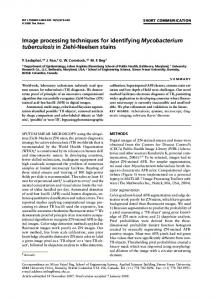
For visualization purposes, each of the regions extracted is illustrated via distinctive colours of the image bands. The joint results of thresholding and masking are displayed in Figure 6.

(a)

Legend Dry exposed area

(b)

(c)

Legend Vegetation Wet, shalow & submerged (Substrate)

Figure 6. Extracted region of river bed: (a) dry exposed area, visualized in the red band overlaid on ortho, (b) shallow submerged and dry exposed visualized in RGB, (c) deep submerged, shallow wet, and dry exposed visualized in RB band and vegetation illustrated in G band.

14

M. S. M. ARIF ET AL.

3.3. Substrate classification based on dominant grain sizes Suitable GLCM and GLDV parameters are considered based on analysis of the statistical distances of individual classes from each other. The window size to be selected for GLCM is critical, which is inter-pixel distance and direction; however eCognition performs this window selection autonomously. The window size for texture measure can be diverse: from being as small as 3 × 3 to as large as 15 × 15 and even larger; and these parameters can have important implications on the classification result. The fine segments classification was implemented on two datasets: the orthomosaic and the classified substrate. For both datasets, different texture parameters were applied. Three test parameters of texture, sample data range, and image band were tested. For the orthomosaic (Figure 7), the first assessment is conducted on the red band with the texture parameters such as GLCM (homogeneity, contrast, and mean), GLDV (mean and entropy), and shape. In the second assessment, the number of parameters for the same red band was increased; with an addition of entropy and dissimilarity as GLCM parameters and the classification was re-conducted. On the third trial, all the three RGB bands were considered, while the number of texture parameters was increased to more measures. The number of texture features applied for GLCM, GLDV, and shape were adjusted based on their relative ability to get separated for each class, hence measures which do not present better isolation among the classes are not considered in the next steps.

Figure 7. Dominant grain classification of orthomosaic based on substrate indexes (Table 1): (a) sample data initiation, (b) RGB image classification via application of texture parameters.

INTERNATIONAL JOURNAL OF REMOTE SENSING

15

Figure 8. Dominant grain classification on substrate layer with RB bands: (a) sample data initiation, (b) RB image classified via application of texture parameters.

On the other hand, the substrate class was investigated for grain classes mapping (Figure 8). The standard sample classes were introduced, and the algorithm was tested. The result was analysed on the bases of reference data, although classification refinement and region merging operations were applied on the neighbourhoods for merging segments of same class. The other testing method used a sample for each class and the segments are then classified based on samples while the similar classified regions are merged. The result for this classification was found to possess various misclassified regions. As input classes, the existing classes from three to nine based on standard substrate indexes were introduced (Table 1). The texture feature considered for sample data are GLCM parameters (entropy, mean, dissimilarity, homogeneity, correlation, and mean) and GLDV parameter (means and entropy), in addition to compactness. The result for the substrate segmentation is shown in Figure 8. For each of the existing classes, three or more objects were selected and introduced as sample data. The reason for selecting multiple samples is to generalize the statistics for existing classes based on grain sizes and textural parameters, and adapt the statistics for a wider selection of class of objects. Finally, a sample result for one of the algorithm implemented in this study for classification of sediment grains and the digitized map of substrate illustrating spatial distribution of grain types are comparatively illustrated in Figure 9. The classes are further segmented and classified in the developed method, which means the homogeneity of grain sizes is further considered, while the manual method has generalized those regions. Considering the image resolution (1 cm/px) and grain sizes within an investigation area, the classes below class 3 (which are smaller than 2 mm) are not considered in this study. Nevertheless, in a small area of the investigation site, class 2 also existed. The spatial distribution of grain classes are depicted in Figure 9.

16

M. S. M. ARIF ET AL.

Figure 9. Comparative illustration of substrate classified map showing spatial distribution of the sediment types based on standard indexes (Table 1): (a) manual mapped dominant grain size classes, (b) result for the developed and executed algorithm in this study. Same colour corresponds the same class in both results.

4. Accuracy assessment and analysis 4.1. Supervised and unsupervised classification Classification accuracy was assessed via the CellArray algorithm in conjunction with the manual estimation. The resulting classification is compared with ground truth data through a series of referenced points. The points are randomly distributed over each class and the user provides values based on the ground truth in the classified map. Finally, the accuracy statistics are provided based on comparison and estimation of thematic class value and ground truth data. An overall accuracy of 70.00% was achieved using the maximum-likelihood method, and overall kappa statistics of 0.6064 (Table 3). The kappa statistic illustrates the measure of difference among the actual agreement of reference data and automated classifier, and the chance between the reference data and a random classifier.

Table 3. Overall accuracy statistics of maximum-likelihood classifications for the test image. Distributed SRP/reference points Class name Unclassified GreenVeg DryGrass Exposed area Submerged Branches Total

Reference totals

Classified totals

Number correct

Producers accuracy

Users accuracy

1 31 24 31 85 27 200

0 14 18 28 69 71 200

– 14 12 25 63 26 140

– 45% 50% 80% 74% 96% –

– 100% 67% 89% 91% 37% –

INTERNATIONAL JOURNAL OF REMOTE SENSING

17

Considering unsupervised classification algorithms, the class boundaries were manually sketched from ground truth data. Next, the results are assessed via ArcGIS and visually compared with the result from the supervised classification. In this assessment, the unsupervised classification was found to have a lower accuracy, requiring a higher amount of manual work for grouping the segments/clusters. Hence, it was disregarded from any further accuracy assessment processes.

4.2. Thresholding and masking The experiment was conducted on various binary cluster images testing diverse clustering methods. The result of this chapter is a segmented orthomosaic. Convolutions were applied on each cluster prior to masking for noise reduction and the removal of excessive information. Convolution parameters were tuned by testing variety of window sizes and kernels. To optimize the computational time, three sections of orthomosaic were masked, including the section defined as the ROI. Each area is selected based on the existence of a variety of end-members for classification, and the degree of complexity of surface types for segmentation of the substrate. This selection does not affect the result for the masking or accuracy estimation; however, it facilitates faster computation and enhances the visualization process of the results. The overall statistics of the portion of orthomosaic processed for segmentation are shown in Figure 10. Accuracy was assessed using a total of 200 random stratified points which were distributed across the ROI, and the class values were provided from the ground truth data. The total accuracy achieved is 96.90% and the overall kappa statistic was 0.852. The total number of points correctly classified is 192 out of 200. This result illustrates the highest accuracy achieved in this study (Figure 11). The comparative analysis of the pixel-based classification algorithms implemented for classifying the orthomosaic into existing members is depicted in Figure 11.

4.3. Substrate classification based on dominant grain sizes A total of 100 points were considered using a stratified distribution across the image and 36 more points were manually digitized for the accuracy assessment of the algorithm as Classification Statistic 12%

32%

11% 20% 9% 36%

Extra class

Substrate

exposed area

Deep submerged

Figure 10. The classified segments statistics and area graphic illustration.

Shallow wet

18

M. S. M. ARIF ET AL.

200

90.58

70

138

96.9

250 200

200

150 100 50

0

Number of Points

Accuracy (%)

Comparative analysis of the Pixel-Based classification 120 100 80 60 40 20 0

0 Unsupervised

Supervised (MLC)

Threshold

Masking

Classification Method Accuracy

Number of points

Figure 11. Comparison of the classification accuracy for pixel-based classification algorithms.

well as the accuracy of each grain class. Overall false classification accuracy obtained is 86.03%, while the overall kappa statistic was 0.8015. However, this result is general and is considered as false accuracy, since this covers the sample area and the regions where there are no ground truth data as well. The area given as sample was measured in GIS from the classified ground truth shapefile, where it was found that 21% of the classified area was manually classified through the sample data. The remaining areas out of the boundaries of the ground truth data map were not considered as suitable for the accuracy assessment. Hence the total accuracy considering the sample area is approximated to a net (true) accuracy of 61%. This percentage could be applied on user and producer accuracy to obtain the accuracy of each class. The gross (false) accuracy assessment result for each of the classes of grain is depicted in Table 4. Correspondingly, in separability analysis of the classes, the class’s value for texture parameters are too close to be distinguished, where in some classes they have a large window area of overlap. The main reason originates from the fact that each class does have consistent texture due to existence of unpredictable grain variety within an identical class. On the other hand, for the accuracy assessment of the segmented substrate with RB band, the results with R and B bands and more parameters for object texture estimation were selected and assessed. Random stratified points were distributed across the classified image, and then the values were provided based on the ground truth sample map. The area assessed for accuracy is the region with valid ground truth data. The additional points which were widely spread all over the image in outer area were removed. Table 4. False accuracy for the grain classes extracted from sample result of substrate. Distributed SRP/reference points Class name Class 3 Class 4 Class 5 Class 6 Class 7 Class 8 Class 9 Unclassified Total

Grain class index 3 4 5 6 7 8 9 – –

Reference total 6 20 11 10 3 8 9 69 136

Classified totals 4 14 9 20 5 7 8 69 136

Number correct 4 12 7 10 2 7 6 69 117

Producers accuracy 66% 60% 63% 100% 66% 87% 67% 100% –

Users accuracy 66% 85% 78% 50% 40% 100% 75% 100% –

INTERNATIONAL JOURNAL OF REMOTE SENSING

19

Table 5. False accuracy result for the grain classes on sample results of orthomosaic. Distributed SRP/reference points Class name Class 3 Class 4 Class 5 Class 6 Class 7 Class 8 Class 9 Unclassified Total

Grain class index 3 4 5 6 7 8 9 – –

Reference total 3 18 15 10 4 12 7 8 77

Classified totals 2 13 13 10 3 26 10 – 77

Number correct 2 13 10 8 3 12 7 – 55

Producers accuracy 66% 72% 67% 80% 75% 100% 100% – –

Users accuracy 100% 100% 76% 80% 100% 47% 70% – –

The overall classification accuracy achieved is 71.43%. This result also falsely includes the sample objects which the user provides. For this purpose, the sample area provided by user was deducted from general assessed points due to which the accuracy falls by 10%. This is because the estimated area of samples was 15% of the total image area, hence the true accuracy is estimated to be 61.4%. On the other hand, due to a lack of ground truth data, the area out of the mapped segments was not assessed. Also the unclassified regions were not considered in this assessment, where misclassifications exist in this class as well. The false accuracy result of the grain classes is illustrated via Table 5. From the classification results for the substrate and the orthomosaic layers, it is found that the result for the substrate layer has more misclassified segments on the area with null values. This is caused when the algorithm considers the null pixels as a class. The reason for this consideration comes from scattered pixels existing in other regions which are introduced as a class to the classifier. The scattered pixels are illustrated with less texture parameters. In the investigated case, class 8 contains grains with large sizes, while the shadowed dark area between gravel pitches is with very low intensity values, and hence not segregated. Thus, more scattered pixels are covered in this class, which makes it the most vulnerable class. In case the scattered areas are considered as unclassified along with null valued pixels, or the segments are provided with smaller-scale value, then the produced result for substrate is expected to have higher accuracy. The number of unclassified area on substrate is less. Conversely, the orthomosaic has vast unclassified area, which affects the result positively for accuracy investigation. This represents that the grain size classes for mid-sized grain objects are of better accuracy. Furthermore, it can be observed that the degree of accuracy for texture-based classification through application of GLCM increases until certain limits, dependent on grain sizes, GLCM and GLDV window sizes, and data formats. In this case, the accuracy can be found to increase from smaller grain classes to bigger. Taking the false accuracy results of both assessments for the producer’s accuracy for grain sizes into account, the chart (Figure 12) is built for better illustration. As observed, the trends are slightly positive for the classes from 3 through 7, though it falls for the classes with larger grain sizes. However, this requires the proper establishment of a relation among the grain size and the window sizes for GLCM and GLDV measures.

20

M. S. M. ARIF ET AL.

"False" producers accuracy for grain classes False Accuracy (%)

120% 100% 80% 60% 40% 20% 0%

Class 3

Class 4

Class 5

Class 6

Class 7

Class 8

Class 9

Grain Classes Producers accuracy Ortho

Producers accuracy Substrate

Figure 12. The user accuracy relation to grain size for both of the substrate and orthomosaic layers.

5. Limitations and recommendations Due to the inherent heterogeneity and diversity of river landscapes, a number of limitations and error sources exist in this study. For further improvement of the results in object-based image analyses, a combination of GLCM and GLDV measures, as well as images with 16 or 32 bit are recommended. Imagery with higher colour depth may improve the texture measures. However, the computational time could be restrictive. Additional combinations of the texture measure and multiple linear regression may also enhance the accuracy of class definitions. Moreover, finer segments enable better segmentation of homogeneous regions, which supports the classification at higher accuracy; therefore, finer segments at smaller scales and sample data for segments with high spatial heterogeneity within the same class is recommended. The grain size variation within a segment can decrease the stability of the algorithm, therefore the optimum window size for averaging needs to be established for heterogeneous image segments with a large variety of grain size types. For minimizing the overlap window of separability among different classes, the finer segments and finding the correlation between the classes and software textural computation algorithm is considered effective. On the other hand, requirement for the site data and samples acquisition across the investigation area is among the drawbacks of the algorithm. One aspect to be considered in future investigations is the existence of deep submerged area, where textural parameters measurement was found to be less effective. We found that in our investigation area more misclassified regions were found within the deep submerged areas. In this study, the best performing measures for GLCM and texture were tested through adjusting the measures based on separability analysis for each of the classes. One of the limitations in this study was the low number of texture measures investigated. Therefore, future studies should focus on testing a wider scope of GLCM, GLDV, and other texture parameters.

6. Conclusions Two methods were evaluated for the semi-automated classification of dominant substrate grain sizes: the first method applied pixel-based and the second object-based

INTERNATIONAL JOURNAL OF REMOTE SENSING

21

classifications. An investigation of pixel-based image analysis provided river cover regions, and a subsequent object-based analysis implemented texture measures for sediment grain classification. The pixel-based assessment adapted supervised classification algorithms as well as a range of unsupervised classification techniques and thresholding algorithms. Although there are no prior rules for the classification types to have better accuracy, the supervised classification method was found to provide higher accuracy in comparison to the unsupervised. The supervised classification provided an overall accuracy of 70%. However, the best overall performance with the highest accuracy for pixel-based classification was achieved via thresholding classification method with overall accuracy of 97% after mask application. Threshold classification was used to successfully segregate different types of cover within the UAV imagery into several regions: dry exposed, shallow water, and merged classes of dry exposed, submerged, and vegetation. The workflow applied in this investigation was tested on several test images, and finally using a 1 cm/px orthomosaic. The proposed method successfully segregates the substrate regions and provided a robust image processing workflow for classification. The accuracy of the algorithm was evaluated in ArcGIS by calculating the segmented areas of pixels and comparing them to field observations which were imported as shape files. The resulting workflow provided 85 ± 10% accuracy in manual method and 90% accuracy in automated method, which is higher than other tested methods of supervised and unsupervised classification. This result is further improved by re-applying the threshold on the green band of the vegetation class for extraction of deep submerged areas. The final result obtained after masking was very satisfactory with 96% correct classification. The proposed workflow is semi-automated and can be implemented via ERDAS IMAGINE 2015, where the user can calibrate the threshold for a given dataset. Masking binary clusters were used to segment the orthomosaic. Kernels were then applied for the removal of scattered pixels, which were considered as a negative factor in correct substrate classification. The kernel application supports the algorithm as an effective tool for classification of mixed-pixel images. Key issues are the resulting accuracy and the amount of information required after kernel application. Therefore, noise reduction via kernels should not affect the accuracy of the algorithm. In this study, it has been established that the thresholding classification system with generation of binary image followed by masking is an effective algorithm with high accuracy for classification of different substrates parts in an aquatic environment, which can replace the conventional manual methods. The results presented for object-based classification of the substrate based on dominant grain sizes indicate that additional in-depth research should be carried out. The texture measures applied should be further assessed. Although the accuracy of the algorithm increases with increasing grain size, the algorithm resulted in a higher number of misclassified regions for larger grain sizes such as class 8 (boulders). This may be mitigated by changing the window size for the GLCM and GLDV. However, it should be noted that the combination of GLCM and GLDV into a single workflow is a highly computationally demanding process. In summary, the work presented provides a workflow comparison of image processing methods for segregating river regions and classifying the dominant sediment grain

22

M. S. M. ARIF ET AL.

size using image processing techniques. The classification procedure for both pixelbased and object-based image analysis using ERDAS IMAGINE and eCognition has been presented, and it was found that satisfactory accuracy can be obtained using UAV aerial imagery to provide maps of the spatial distribution of the dominant substrate.

Disclosure statement No potential conflict of interest was reported by the authors.

ORCID Jeffrey A. Tuhtan

http://orcid.org/0000-0003-0832-7334

References Allan, J. D. 1995. Stream Ecology; Structure and Function of Running Waters, 388. New York: Chapman & Hall. ISBN:O-4 12-35530-2. Bangen, S. B., J. M. Wheaton, N. Bouwes, B. Bouwes, and C. Jordan. 2013. “A Methodological Intercomparison of Topographic Survey Techniques for Characterizing Wadeable Streams and Rivers.” Geomorphology. doi:10.1016/j.geomorph.2013.10.0100.010. Carbonneau, P. E., S. N. Lane, and N. Bergeron. 2006. “Feature Based Image Processing Methods Applied to Bathymetric Measurements from Airborne Remote Sensing in Fluvial Environments.” Earth Surface Processes and Landforms 31: 1413–1423. doi:10.1002/esp.1341. Carbonneau, P. E., S. N. Lane, and N. E. Bergeron. 2004. “Catchment-Scale Mapping of Surface Grain Size in Gravel Bed Rivers Using Airborne Digital Imagery.” Water Resources Research 40: W07202. doi:10.1029/2003WR002759. eCognition Developer 8. 2009. User Guide. Document version 1.2.0. Munich: Definiens AG. ERDAS Inc. 1999. ERDAS Field Guide. 5th ed. Atlanta, GA: ERDAS inc. Gillavry, E. M. 1998. Textural Pattern Recognition: Distinguishing between Occupation Densities in the Centre of Dar Es Salaam. Utrecht: Department of Cartography, University of Utrecht. Haralick, R. M. 1979. “Statistical and Structural Approaches to Texture.” Proceedings of the Institute of Electrical and Electronics Engineers 67 (5): 786–804. doi:10.1109/PROC.1979.11328. Haralick, R. M., K. Shanmugam, and I. Dinstein. 1973. “Textural Features for Image Classification.” IEEE Transactions on Systems, Manual and Cybernetics 3 (6): 610–621. Hicks, D. M. 2012. “Remotely Sensed Topographic Change in Gravel Riverbeds with Flowing Channels.” In Gravel-Bed Rivers: Processes, Tools, Environments, edited by M. Church, P. M. Biron, and A. G. Roy. Chichester: John Wiley & Sons. doi:10.1002/9781119952497.ch23. Hugenholtz, C. H., K. Whitehead, O. W. Brown, T. E. Barchyn, B. J. Moorman, A. Leclair, K. Riddell, and T. Hamilton. 2013. “Geomorphological Mapping with a Small Unmanned Aircraft System (sUAS): Feature Detection and Accuracy Assessment of a Photogrammetrically-Derived Digital Terrain Model.” Geomorphology 194: 16–24. doi:10.1016/j.geomorph.2013.03.023. Lillesand, T. M., and R. W. Kiefer. 1994. Remote Sensing and Image Interpretation, xvi + 750. 3rd ed. Chichester: John Wiley & Sons. ISBN:0 471 30575 8 (pb). Maddock, I. 1999. “The Importance of Physical Habitat Assessment for Evaluating River Health.” Freshwater Biology 41: 373–391. doi:10.1046/j.1365-2427.1999.00437.x. Meinel, G., and M. Neubert. 2004. “A Comparison of Segmentation Programs for High Resolution Remote Sensing Data.” Geo-Imagery Bridging Continents. XXth ISPRS Congress (ISPRS International Archives of the Photogrammetry, Remote Sensing and Spatial Information Sciences; vol. XXXV, Part B4), Istanbul, Turkey. July 12–23, 1097–1102. Mihran, T., and K. J. Anil. 1993. Texture Analysis, Handbook of Pattern Recognition & Computer Vision. River Edge: World Scientific.

INTERNATIONAL JOURNAL OF REMOTE SENSING

23

Otsu, N. 1979. “A Threshold Selection Method from Gray-Level Histograms.” IEEE Transactions on Systems, Manual and Cybernetics 9 (1): 62–66. doi:10.1109/TSMC.1979.4310076. Schneider, M., M. Noack, T. Gebler, and I. Kopecki. 2010. Handbook for the Habitat Simulation Model. CASiMiR-Fish. Stuttgart: Institute für Wasserbau, Universität Stuttgart and sje Ecologial Engingeering GmbH. Schowengerdt, R. A. 2007. Remote Sensing, 515. 3rd ed. United States: Academic Press Elsevier. ISBN: 9780123694072. Tillmann, C. 2012. “Supervised Classification and Change Detection of Agricultural Land Use in the Forest Steppe Zone of West Siberia Using Multitemporal Satellite Imagery.” Master thesis in the subject Landscape Ecology, University of Münster. Vos, C. C., C. J. F. Braak, and W. Nieuwenhuizen. 2000. “Incidence Function Modelling and Conservation of the Tree Frog Hyla Arborea in the Netherlands.” Ecological Bulletins 48: 165–180. Wheaton, J. M., J. Brasington, S. E. Darby, and D. Sear. 2010. “Accounting for Uncertainty in DEMs from Repeat Topographic Surveys: Improved Sediment Budgets.” Earth Surface Processes and Landforms 35 (2): 136–156. doi:10.1002/esp.1886. Zhi-Hua, Z., L. Hang, and Y. Qiang. 2007. “Advanced in Knowledge Discovery and Data Mining.” 11th Pacific-Asia Conference, PAKKD 2007, Nanjin, China. ISBN:9783540717010 • 9783540717003. doi:10.1007/978-3-540-71.