International Journal of Computer Science & Information Technology (IJCSIT), Vol 3, No 3, June 2011
AN LMS BASED BLIND SOURCE SEPARATION ALGORITHM USING A FAST NONLINEAR AUTOCORRELATION METHOD Behzad Mozaffari Tazehkand Faculty of Electrical and Computer Engineering University of Tabriz, Tabriz, Iran
[email protected]
ABSTRACT Blind source separation (BSS) is the technique that anyone can separate the latent data from their mixtures without any knowledge about the mixing process, but using some statistical properties of original source signals. In this paper we will use the nonlinear autocorrelation function as an object function to separate the source signals from the mixing signals. Maximization of the object function using the LMS algorithm will be obtained the coefficients of a basic linear filter which separate the source signals. To calculating the performance of proposed algorithm two parameters such as Performance Index (PI) and Signal to Interference Ratio (SIR) will be used. It will be shown that the proposed algorithm gives better results than other method such as Newton method which has been proposed by Shi.
KEYWORDS BSS, LMS Algorithm, Newton Method, Nonlinear Autocorrelation, Speech Processing
1. INTRODUCTION Blind source separation (BSS) is the technique that anyone can separate the original signals or latent data from their mixtures without any knowledge about the mixing process, but using some statistical properties of latent or original source signals. Blind source separation (BSS) using Independent Component Analysis (ICA) has attracted great deal of attention in recent years. Important applications such as pattern recognition, speech recognition systems, speech enhancement, speech and image separation, wireless communication, image processing, telecommunications, data mining, and biomedical signal analysis and processing has been carried out using ICA [1-2]. The main objective of ICA is to identify independent sources using only sensor observation datum which are linear mixtures of unobserved independent source signals [3-5]. In fact, the ICA is an algorithm for solving the BSS problems, which assumes the source signals are non-Gaussian. The standard formulation of ICA requires at least as many sensors as sources [4]. Many algorithms for BSS have been proposed by researchers using the statistical properties of original signals such as non-gaussianity [6-14], smoothness [9,15], linear autocorrelation [10,16-17], temporal algorithms [18-20], nonstationarity [21-23], sparsity [24-27], nonnegativity [28-29] and nonlinear autocorrelation [30-33]. Tinati et al proposed a comparison method for speech signal orthogonality in wavelet and timefrequency domains [34]. Tinati et al proposed a new algorithm for selecting best wavelet packet node using LMM-EM model, finally they could obtain best results about estimation of mixing matrix [35-36]. They apply LMM model for speech mixture signals in wavelet packet domain using long-term Analysis. They also applied the wavelet packet transform in their proposed algorithm and obtained the best results [37]. DOI : 10.5121/ijcsit.2011.3315
218
International Journal of Computer Science & Information Technology (IJCSIT), Vol 3, No 3, June 2011
Zhenewi Shi et al proposed a nonlinear autocorrolation of source signals for solving the BSS problems. They proposed a fixed point algorithm to solve the BSS problem based on nonlinear autocorrelation also they showed anyone can solve the BSS problem by maximizing the nonlinear temporal autocorrelation of source signals [31]. Zhenewi Shi et al also proposed a fast method for solving the BSS problems using the non-Gaussianity and nonlinear temporal autocorrelation structure assumption. They applied Newton algorithm as an iterative method for signal separation [32]. In this paper we use the nonlinear autocorrelation method based on LMS algorithm to source signal separation. The obtained results are compared with other reported results. Using the signal to noise ratio and the performance index parameter it will be shown that our obtained results are better than the Shi algorithm.
2. BACKGROUND MATERIALS 2.1. Independent Component Analysis Independent component analysis is a statistical method expressed as a set of multidimensional observations that are combinations of unknown variables [1-2,4]. These underlying unobserved variables are called sources and they are assumed to be statistically independent with respect to each other. The linear ICA model is expressed as the following equation: X(t)=A×S(t)
(1) T
th
Where X(t)=[x1(t),x2(t),x3(t),…,xM(t)] is an observed vector and xi(t) is the i mixture signal. A=[aij]M×N is an unknown M×N mixing matrix that operates on statistically independent unobserved variables which is defined as the following vector: S(t)=[s1(t),s2(t),s3(t),…,sN(t)]T Where again si(t) is the ith source signal. It is assumed that any entry of mixing matrix A has a constant value, in other words the ICA system is an LTI system and also we assumed that the source signals have zero mean and unit energy or variance. In the case of an equal number of sources and sensors, (M=N), a number of robust approaches using independent component analysis have been proposed by many researchers [38-39]. In this case ICA method estimates the inverse or pseudo inverse of mixing matrixes as W.
2.2. Whitening Filter One of the important assumption of ICA method is that the observation data or signals must be have unit variance and be uncorrelated with each other. Therefore the observations signals must be processed using whitening filter such ‘V’ vector as follows: X% ( t ) = V × X ( t )
(2)
Where the ‘V’ vector can be obtained as the following equations: V =D
− 21
× ET
(3)
If we define the covariance matrix of observation data as: C X = E{ X × X T }
(4)
Where ‘D’ is the diagonal matrix defined as: D=diag(d1 d2 … di … dN) where ‘di’ is the ith eigenvalue of the covariance matrix of observation data and ‘E’ is the corresponding eigenvector matrix.
219
International Journal of Computer Science & Information Technology (IJCSIT), Vol 3, No 3, June 2011
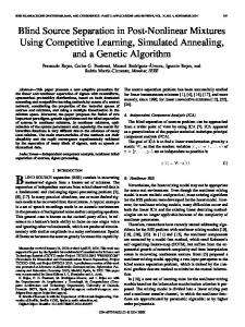
2.3. Nonlinear Autocorrelation to BSS Problem We assume that the observation data obtained by sensors is modeled using (1) where the ‘A’ is N×N square mixing matrix and it’s each entries is a constant real numbers. We also assume that the original signals are mutually independent and have a nonlinear autocorrelation with each other. w1 x1(t) xi(t) xN(t)
wi
+
ŝi(t)
wN
Figure 1. Basic Linear Instantaneous Filter for BSS Using a basic linear instantaneous filter as shown in figure (1) with the tap gain vector as W=[w1,w2,…,wN]T anyone can estimate the desired source signal ŝi(t) as the following equation. Sˆ i ( t ) = W T × X ( t )
(5)
Where ‘W’ is the unknown vector that must be obtained using an optimal method. With the definition of τ as some lag constant we can use the delayed version of the estimated source signal to obtaining the autocorrelation function of estimated source signal as: Sˆ i ( t − τ ) = W T × X ( t − τ )
(6)
To obtaining the ‘W’ vector we will use the nonlinear autocorrelation [31-32] of estimated signals as an object function and maximizing it respect to have unit energy for the ‘W’ vector. The object function can be written as:
max ψ ( W3) = E{ G( Sˆ i ( t ))G( Sˆ i ( t − τ ))} = E{ G( W T X% ( t ))G( W T X% ( t - τ ))} 1 424
(7)
W =1
Where X̃ (t) is the whitened form of the observation data given by (2) and the ‘G’ operator is a differentiable nonlinear function, which measures the nonlinear autocorrelation degree of the estimated source signal. This nonlinear function can be choice such as G(x)=x2 and G(x)=logcosh(x).
3. PROPOSED METHOD 3.1. Learning Method Using the LMS Algorithm To maximizing the objective function defined by (7), we apply the LMS method therefore the weight vector defined as ‘W’ can be obtained as following equations: W ( k + 1) ←W ( k )− µ
∂ψ W , W← ∂W W
(8)
∂ψ = E{ g ( Sˆ ( t ))G( Sˆ ( t − τ )) X% ( t ) + G( Sˆ ( t ))g ( Sˆ ( t − τ )) X% ( t − τ )} ∂W
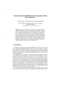
Where ‘g’ function is the derivative of ‘G’. Using the above equations given by (8) we can summarize the proposed algorithm as figure (2).
220
International Journal of Computer Science & Information Technology (IJCSIT), Vol 3, No 3, June 2011
Input Mixture Signals: X(t)=
[x1(t),x2(t),x3(t),…,xN(t)]T
Obtaining the whitened form of X ( t ) a s X% ( t )
Initialize the ‘W’ vector
W (k +1)← W (k )− µ
∂ψ ∂W
Normalize the ‘W’ vector
Condition is accepted?
NO
YES
Calculate Corresponding Source Signals
Figure 2. The Proposed Algorithm to Obtaining the Source Signals
3.2. Simulation Results As described in proposed method, we apply the LMS algorithm for source signal separation such as speech and ECG data with considering the nonlinear functions G(x)=x2 and G(x)=log(cosh(x)). To measuring the degree of accuracy of source separation in proposed algorithm two parameters such as 1) Signal to Interference Ratio (SIR) and 2) Performance Index (PI) are considered. These parameters are defined as the following equations [32]:
SIRi = 10log(
PI =
( si ( t ))2 ) ( si ( t ) − s%i ( t ))2
n n pij pij 1 n n { ( − 1 ) + ( − 1 )} ∑ ∑ ∑ ∑ n2 i =1 j =1 maxk pik j =1 i =1 maxk pkj
(9)
(10)
In the PI parameter pij is the i,jth element of P=W×V×A matrix. This matrix is the matrixes which can be separate the source signals. The larger value of PI parameter indicates that the separation is done in poorer. Example: We consider 4 speech signals as shown in figure (3) with sampling rate 16000 sample per second which selected from TIMIT database. It is assumed that these source signals are zero mean and unit variances. These signals are mixed using a random mixing matrix and the mixing signals are obtained as an observation signals. The mixing signals are plotted in figure (4). 221
International Journal of Computer Science & Information Technology (IJCSIT), Vol 3, No 3, June 2011
Amplitude
We apply the proposed algorithm and the estimated source signals are computed which shown as figure (5). 10 0
Amplitude
-10
0
0.1
0.2
0.3
0.4
0.5 0.6 time(sec)
0.7
0.8
0.9
1
0
0.1
0.2
0.3
0.4
0.5 0.6 time(sec)
0.7
0.8
0.9
1
0
0.1
0.2
0.3
0.4
0.5 0.6 time(sec)
0.7
0.8
0.9
1
0
0.1
0.2
0.3
0.4
0.5 0.6 time(sec)
0.7
0.8
0.9
1
10 0
Amplitude
-10
10 0
Amplitude
-10
10 0 -10
Amplitude
Amplitude
Amplitude
Amplitude
Figure 3. Speech Source Signals 5 0 -5
0
0.1
0.2
0.3
0.4
0.5 0.6 time(sec)
0.7
0.8
0.9
1
0
0.1
0.2
0.3
0.4
0.5 0.6 time(sec)
0.7
0.8
0.9
1
0
0.1
0.2
0.3
0.4
0.5 0.6 time(sec)
0.7
0.8
0.9
1
0
0.1
0.2
0.3
0.4
0.5 0.6 time(sec)
0.7
0.8
0.9
1
10 0 -10
10 0 -10
10 0 -10
Amplitude
Amplitude
Amplitude
Amplitude
Figure 4. Mixing Signals 10 0 -10
0
0.1
0.2
0.3
0.4
0.5 0.6 time(sec)
0.7
0.8
0.9
1
0
0.1
0.2
0.3
0.4
0.5 0.6 time(sec)
0.7
0.8
0.9
1
0
0.1
0.2
0.3
0.4
0.5 0.6 time(sec)
0.7
0.8
0.9
1
0
0.1
0.2
0.3
0.4
0.5 0.6 time(sec)
0.7
0.8
0.9
1
10 0 -10
10 0 -10
10 0 -10
Figure 5. Estimated Speech Signals 222
International Journal of Computer Science & Information Technology (IJCSIT), Vol 3, No 3, June 2011
Performance Index
0.2 LMS Algorithm Newton Algorithm
0.15 0.1 0.05 0
1
2
3
4
5 6 iteration
7
8
9
10
Figure 6. PI Parameter with τ=13 for LMS and Newton Methods Table 1. SIR parameter of Estimated Speech Signals for both methods Method
SIR1(dB) SIR2(dB) SIR3(dB) SIR4(dB)
Shi
22.2134
26.6651
38.3949
21.9902
Proposed
28.0435
26.4293
38.4228
31.8080
To comparison of the proposed algorithm with the Shi algorithm (Newton Method) [32] Performance Index (PI) and Signal to Interference Ratio (SIR) parameters are computed to both methods. In figure (6) the PI Parameter for both method are plotted and it is shown that the value of PI parameter in LMS Method is better than Newton method. Also, in table (1) SIR parameter for the estimated source signal are shown in both algorithm and again the obtained results are better than other algorithm.
4. CONCLUSIONS In this paper the nonlinear autocorrelation function as an object function is used to solving the BSS problem. With maximizing of the object function using LMS algorithm the coefficients of a basic linear filter are obtained and therefore the separation of source signal is done. To obtaining of accuracy of the proposed algorithm the performance index and SIR parameter are calculated and the obtained results are compared with the Newton method. It is shown that the proposed algorithm gets better results than the other method.
REFERENCES [1]
McKeown, M., Hansen, L. K., Sejnowski, T. J.,”Independent Component Analysis for fMRI: What is Signal and what is Noise?”, Current Opinion in Neurobiology, Vol. 13(5), pp. 620-629, 2003
[2]
Karlsen B., Sorensen, H. B., Larsen, J., Jackobsen, K. B., “Independent Component Analysis for Clutter Reduction in Ground Penetrating Radar Data”, Proceedings of the SPIE, AeroSense 2002, Vol. 4742, pp. 378-389, SPIE, 2002
[3]
J.-F. Cardoso, “Blind signal separation: Statistical principles”, Proc. IEEE, vol. 86, pp. 2009– 2025, Oct. 1998.
[4]
P. Comon, “Independent component analysis — A new concept?”, Signal Process., vol. 36, pp. 287–314, 1994.
[5]
T.W. Lee, “Independent Component Analysis: Theory and Applications.”, Boston, MA: Kluwer, 1998.
[6]
S.I. Amari, A. Cichocki, H.H. Yang, “A new learning algorithm for blind source separation”, Advances in Neural Information Processing Systems, Vol. 8, 1996, pp. 757–763. 223
International Journal of Computer Science & Information Technology (IJCSIT), Vol 3, No 3, June 2011 [7]
A. Bell, T. Sejnowski, “An information-maximization approach to blind separation and blind deconvolution”, Neural Computation, Vol. 7, Issue 6, 1995, pp. 1129–1159.
[8]
J.-F.Cardoso, B.H. Laheld, “Equivariant adaptive source separation”, IEEE Transactions on Signal Processing, Vol. 44, Issue 12, 1996, pp. 3017–3030.
[9]
A.Cichocki, S.-I. Amari, “Adaptive Blind Signal and Image Processing: Learning Algorithms and Applications”, Wiley, NewYork, 2002.
[10]
A. Hyvärinen, “Fast and robust fixed-point algorithms for independent component analysis”, IEEE Transactions on Neural Networks, Vol. 10, Issue 3, 1999, pp. 626–634.
[11]
A.Hyvärinen, J. Karhunen, E. Oja, “Independent Component Analysis”, Wiley, New York, 2001.
[12]
C. Jutten, J. Herault, “Blind separation of sources, part I: an adaptive algorithm based on neuromimetic architecture”, Signal Processing Vol. 24, 1991, pp. 1–10.
[13]
T.W. Lee, M. Girolami, T. Sejnowski, “Independent component analysis using an extended infomax algorithm for mixed sub-Gaussian and super-Gaussian sources”, Neural Computation Vol. 11, Issue 2, 1999, pp. 417–441.
[14]
Z.Y. Liu, K.C. Chiu, L. Xu, “One-bit-matching conjecture for independent component analysis”, Neural Computation, Vol. 16, 2004, pp. 383–399.
[15]
A.K. Barros, A .Cichocki, “Extraction of specific signals with temporal structure”, Neural Computation” Vol. 13, Issue 9, 2001, pp.1995–2003.
[16]
L. Tong, R.W. Liu, V. Soon, Y.F. Huang, “Indeterminacy and identifiability of blind identification”, IEEE Transactions on Circuits and Systems, Vol. 38, Issue 5, 1991, pp. 499–509.
[17]
A. Belouchrani, K.A. Meraim, J.F. Cardoso, E.Moulines, “A blind source separation technique based on second order statistics”, IEEE Transactions on Signal Processing, Vol. 45, Issue 2, 1997, pp. 434–444.
[18]
J.V. Stone, “Blind source separation using temporal predictability”, Neural Computation, Vol. 13, 2001, pp. 1559–1574.
[19]
S. Douglas, S.C. Sawada, H. Makino, “A spatio-temporal fastICA algorithm for separating convolutive mixtures”, ICASSP’05, Vol. 5, 2005, pp. 165-168
[20]
Huan Tao, Jian-yun Zhang, Lin Yu, “A New Step-Adaptive Natural Gradient Algorithm for Blind Source Separation”, Springer Series, Vol. 344, 2006, pp.35-40
[21]
A.Hyvärinen, “Blind source separation by nonstationarity of variance: a cumulant-based approach”, IEEE Transactions on Neural Networks, Vol. 12, Issue 6, 2001, pp. 1471–1474.
[22]
K. Matsuoka, M. Ohya, M. Kawamoto, “A neural net for blind separation of nonstationary signals”, Neural Networks, Vol. 8, Issue 3, 1995, pp. 411–419.
[23]
D.-T. Pham, J.F. Cardoso, “Blind separation of instantaneous mixtures of nonstationary sources”, IEEE Transactions on Signal Processing, Vol. 49, Issue 9, 2001, pp. 1837–1848.
[24]
Y.Q. Li, A. Cichocki, S.I. Amari, “Analysis of sparse representation and blind source separation”, Neural Computation, Vol. 16, Issue 6, 2004, pp. 1193–1234.
[25]
M.S. Lewicki, T.J. Sejnowski, “Learning overcomplete representations”, Neural Computation, Vol. 12, Issue 2, 2000, pp. 337–365.
[26]
Z. Shi, H. Tang, Y. Tang, “Blind source separation of more sources than mixtures using sparse mixture models”, Pattern Recognition Letters, Vol. 26, Issue 16, 2005, pp. 2491–2499.
[27]
M. Zibulevsky, B.A. Pearlmutter, “Blind source separation by sparse decomposition in a signal dictionary”, Neural Computation, Vol. 13, 2001, pp. 863–882.
[28]
E. Oja, M.D. Plumbley, “Blind separation of positive sources by globally convergent gradient search”, Neural Computation, Vol. 16, Issue 9, 2004, pp. 1811–1825. 224
International Journal of Computer Science & Information Technology (IJCSIT), Vol 3, No 3, June 2011 [29]
M.D. Plumbley, E. Oja, A “non-negative PCA algorithm for independent component analysis”, IEEE Transactions on Neural Networks, Vol. 15, Issue 1, 2004, pp. 66–76.
[30]
Z. Shi, C. Zhang, “Nonlinear innovation to blind source separation”, Neurocomputing, Vol. 71, 2007, pp. 406–410.
[31]
Z. Shi, Z. Jiang, F. Zhou, “A fixed-point algorithm for blind source separation with nonlinear autocorrelation”, Journal of Computational and Applied Mathematics, Vol. 223, Issue 2, 2008, pp. 908-915.
[32]
Zhenwei Shi, Changshui Zhang, “Fast nonlinear autocorrelation algorithm for source separation”, Pattern Recognition, 2008, doi: 10.1016/j.patcog.2008.12.025.
[33]
Zhenwei Shi, Zhiguo Jiang, Fugen Zhou, Jihao Yin, “Blind source separation with nonlinear autocorrelation and non-Gaussianity”, Journal of Computational and Applied Mathematics, Vol. 229, Issue 1, 2009, pp. 240-247.
[34]
M.A. Tinati, B. Mozaffari, “Comparison of Time-frequency and Time-scale analysis of speech signals using STFT and DWT”, WSEAS Transaction on Signal Processing, Issue 1, Vol. 1, Oct. 2005, pp. 11-16.
[35]
B. Mozaffari, M.A. Tinati, “Blind Source Separation of Speech Sources in Wavelet Packet Domains Using Laplacian Mixture Model Expectation Maximization Estimation in Overcomplete- Cases”, Journal of Statistical Mechanics: Theory and Experiments An IOP and SISSA Journal, 2007, pp. 1-31.
[36]
M.A. Tinati, B. Mozaffari, “A Novel Method to Estimate Mixing Matrix under Over-complete Cases in Wavelet Packet Domain”, ICCCE08, 2008, pp.493-496.
[37]
B. Mozaffari, M.A. Tinati, A Novel Blindly Mixing Matrix Estimation of Speech Source Signals Using Short Time-Wavelet Packet Analysis by Simple Laplacian Model in Over-Complete Cases, MICC’09, 2009, pp. 597-602.
[38]
A.K. Barros, H. Kawahara, A. Cichocki, S. Kojita, T. Rutkowski, M. Kawamoto, and N. Ohnishi, “Enhancement of speech signal embedded in noisy environment using two microphones”, In proceedings of the second international workshop on ICA and BSS, ICA2000, pp. 423-428.
[39]
M.A. Tinati, B. Mozaffari, “A Novel Method for Noise Cancellation of Speech Signals Using Wavelet Packets”, the 7th International Conference on Advanced Communication Technology, ICACT 2005, Vol. 1, pp. 35–38.
Authors Behzad Mozaffari Tazehkand was born in 1968 in Iran. He received his B.S. degree in 1993 from University of Tabriz and his M.S. degree in 1996 from K.N.Toosi University of Technology. Also he received his Ph.D. degree in 2007 in electrical communication engineering in the University of Tabriz. His research interests are signal processing and speech processing and wireless communication.
225