An Optimized DBN-Based Mode-Focussing Particle Filter S´everine Dubuisson and Christophe Gonzales Laboratoire d’Informatique de Paris 6, Universit´e Pierre et Marie Curie, France
[email protected]
Abstract
y1 x1
p(xt+1 |xt )p(xt |y1:t )
xt x2t+1
x2t yt2
2 yt−1
yt1
1 yt−1
yt3
3 yt−1
time slice t − 1
(b)
1 yt+1
x3t+1
x3t
x3t−1
2 yt+1
x1t+1
x1t
x1t−1
time slice t
3 yt+1
time slice t + 1
Figure 1. (a) A Markov chain for state estimation. (b) A DBN.
with p(xt+1 |xt ) the transition corresponding to function ft+1 and p(yt+1 |xt+1 ) the likelihood corresponding to ht+1 . Probability p(xt+1 |y1:t+1 ) can be computed similarly with prediction and correction steps defined by: R p(xt+1 |y1:t ) = xt p(xt+1 |xt )p(xt |y1:t )dxt (3)
Articulated object tracking is an important task in computer vision. Its applications include in particular gesture recognition, human tracking and event detection. Unfortunately, tracking articulated structures with accuracy and within a reasonable time is computationally challenging due to the high dimensionality of the state and observation spaces. In this paper, we tackle this problem using Sequential Monte Carlo methods (a.k.a. Particle Filter – PF). Essentially, this framework [3] aims at estimating a state sequence {xt }t=1,...,T , whose evolution is given by xt+1 = ft+1 (xt , nxt+1 ), from a set of observations {yt }t=1,...,T related to the state by yt+1 = ht+1 (xt+1 , nyt+1 ). Usually, ft+1 and ht+1 are nonlinear functions, and nxt+1 and nyt+1 are i.i.d. noise sequences. This problem is naturally represented by the Markov chain of Fig. 1.(a). From a probabilistic point of view, it amounts to estimate, for any t, either i) p(x1:t |y1:t ) or ii) p(xt |y1:t ), where x1:t denotes the tuple (x1 , . . . , xt ). The first quantity can be computed by iteratively using Eq. (1) and (2), which are referred to as a prediction step and a correction step respectively. =
....
x2
x2t−1
1. Introduction
p(x1:t+1 |y1:t )
yt
(a)
We propose an original particle filtering-based approach combining optimization and decomposition techniques for sequential non-parametric density estimation defined in high-dimensional state spaces. Our method relies on Annealing to focus on the correct distributions and on probabilistic conditional independences defined by Dynamic Bayesian Networks to focus samples on their modes. After proving its theoretical correctness and showing its complexity, we highlight its ability to track single and multiple articulated objects both on synthetic and real video sequences. We show that our approach is particularly effective, both in terms of estimation errors and computation times.
p(x1:t+1 |y1:t+1 ) ∝
y2
p(xt+1 |y1:t+1 ) ∝
p(yt+1 |xt+1 )p(xt+1 |y1:t ).
(4)
Basically, PF aims at approximating the above distributions using weighted samples. Thus, Eq. (3) and (4) are (i) (i) estimated by samples {xt+1 , wt+1 } of N possible realiza(i) tions of the state xt+1 called particles. In the prediction step (i) (i) (Eq. (3)), PF propagates the particle set {xt , wt } using a (i) proposal function q(xt+1 |x1:t , yt+1 ); in the correction step (Eq. (4)), PF weights the particles using a likelihood func(i)
(i)
(i)
p(x
(i)
(i)
|x
)
tion, so that wt+1 ∝ wt p(yt+1 |xt+1 ) (i) t+1(i) t , q(xt+1 |x1:t ,yt+1 ) PN (i) with i=1 wt+1 = 1. The particles can then be resampled: those with the highest weights are duplicated, while the others are eliminated. The estimation of the posterior density PN (i) p(xt+1 |y1:t+1 ) is then given by i=1 wt+1 δx(i) (xt+1 ), t+1
(i)
where δx(i) are Dirac masses centered on particles xt+1 . t+1 Of course, PF can approximate Eq. (1) and (2) in a similar (i) (i) way using weighted samples of tuples (x1 , . . . , xt+1 ). As shown in [6], the number of particles necessary for a good estimation of the above densities grows exponentially with the dimension of the state space, hence making PF’s
(1)
p(yt+1 |xt+1 )p(x1:t+1 |y1:t ) (2) 1
basic scheme unusable in real-time. In the literature, different variants of PF have been proposed to cope with highdimensional spaces. They can be roughly divided into three categories: i) those that reduce the state space dimension by approximating it; ii) those that reduce it by making local searches; and iii) those that exploit natural independences in the state space to decompose it into a set of sub-spaces of reasonable sizes where PF can be applied. Here, for accuracy reasons, we focus on the last two approaches. Among the local search-based approaches, let us cite the popular Annealed Particle Filter (APF) [2] that consists of adding annealing iterations (or layers) to PF’s resampling step in order to better diffuse particles in the state space. Among the third type of approaches, Partitioned Sampling (PS) [5] decomposes the state space as a Cartesian product of conditionally independent subspaces and iterates PF over all of them. A similar idea based on Dynamic Bayesian Networks (DBN) [7] is exploited in [4]: the proposal function q is decomposed as the product of the conditional densities in each node of the network, and PF is applied sequentially on each node following a topological order of the DBN. These two approaches are combined in [9] to define an algorithm for PF totally integrated into a DBN. The work described in [1] is probably the closest to ours: a parallel algorithm of PF is described that uses the same joint probability in the DBN to reduce the number of particles. The state space is divided into subspaces in which the particles are independently generated by several proposal densities q. This approach enables to easily choose q to sample each subspace. However, it requires a specific independence structure in the DBN that limits the generalization of the algorithm. In this paper, we propose to significantly refine both PS and APF by fully exploiting conditional independences in the state space defined by DBNs. More precisely, we will show that, using DBNs, some permutations of PS’s substates can be performed that focus the samples on the modes of the distributions. When combined with APF, this scheme proves particularly effective, both to significantly reduce estimation errors and to keep computation times low. The paper is organized as follows. In Section 2, we recall the basics of APF and PS. In Section 3, we describe our approach, prove its correctness and show its computational complexity. Using experiments on synthetic and real video sequences, Section 4 highlights the efficiency of the method both in terms of estimation errors and computation times. Finally, we conclude and give perspectives in Section 5.
2. Basics of PS and APF The key idea of PS is that the state and observation spaces X and Y can often be naturally decomposed as X = X 1 × · · · × X P and Y = Y 1 × · · · × Y P where conditional independences between subspaces (X i , Y i ) can be exploited so that the sequential application of PF on each of
them provides samples over (X , Y) estimating p(xt |y1:t ). As these subspaces are “smaller”, the distributions to estimate have fewer parameters than those defined on (X , Y), which significantly reduces the number of particles needed for their estimation and, thus, speeds up the computations. (i),j (i),−j More precisely, let (ˆ xt , x t ) denote the particle with (i) (i) the same state as x ˆt on part j and the same as xt on the (i) other parts. Then, given a sample {xt } at time t, PS first (i),1 (i),−1 uses PF to compute sample {ˆ xt+1 , xt )} where only the first part is propagated/corrected. Then, with this new sample, PF is applied on the second part, and so on (see [5] for details). As an example, to track a human body, X can be naturally decomposed as X torso ×X left arm ×X right arm where, given the position of the torso, the left and right arm positions are independent. PS then first applies PF on the torso, then on the left arm and finally on the right arm. However, by multiplying the number of subspaces, we also multiply the resampling steps which, in turn, increases the noise in the estimation process and decreases its accuracy. Quite differently, APF increases the accuracy of PF by exploiting a local search process in order to find the modes of the distributions. More precisely, after applying PF on the whole space X , it explores the neighborhood of the particles to move them toward the modes. To do so, it alternates some form of weighted resampling that guarantees some survival rate of the particles with iterations of PF. This process is called annealing. Of course, APF can be combined with PS by substituting each iteration of PF over X by one of PS. This algorithm is denoted by PS-APF.
3. A Particle Filter with substate permutation The algorithm we propose in this paper heavily relies for its correctness on the DBN’s independence model, a.k.a. dseparation [8]. An example of a DBN is shown in Fig. 1.b. Basically, each node of a DBN represents a random variable and is assigned its probability distribution conditionally to its parents in the graph. The DBN represents the joint distribution of all its nodes as the product of all their conditional distributions. Hence, two nodes, say xit and xjs are dependent conditionally to a set of nodes Z if and only if there exists a chain {c1 = xit , . . . , cn = xjs } linking xit and xjs in the DBN such that i) for every node ck such that the DBN arcs are ck−1 → ck ← ck+1 , either ck or one of its descendants is in Z; and ii) none of the other nodes ck belongs to Z. Such a chain is called active. This is the d-separation criterion [8]. In our body tracking problem, given the position of the body in the past, as both arms are independent conditionally to the position of the torso, p(torso, left arm, right arm) = p(torso) × p(left arm|torso) ×p(right arm|torso), justifying that the DBN of Fig. 1.b models this tracking problem if x1t , x2t , x3t represent the torso and the left and right arms respectively.
PS, as introduced in [5], did not rely on DBNs. However, the latter can be used to justify its correctness. Actually, if, by d-separation, for any j ∈ {1, . . . , P }, xjt is independent j−1 P 1 , xjt−1 ), of (xj+1 t−1 , . . . , xt−1 ) conditionally to (xt , . . . , xt j then each iteration of PF over one substate xt samples over P a distribution which is independent of (xj+1 t−1 , . . . , xt−1 ). This is precisely what is needed to ensure that, after iterating over the P parts of the object, PS and PS-APF have both sampled over distribution p(xt |y1:t ). For instance, in the DBN of Fig. 1.b, x1t , x2t , x3t satisfy the above property and, thus, PS-APF can be used to perform PF first on the torso, then on the left arm and finally on the right arm. Our algorithm exploits d-separation, first, to identify independent tracking subproblems where PF can be performed in parallel and, second, to mix their results in a most efficient way. More formally, we will assume that, within each time slice, the DBN structure is a directed tree (or a forest if we track multiple objects), i.e., there do not exist nodes xit , xjt , xkt with the graph topology xit → xjt ← xkt . In addition, we will assume that arcs across time slices link similar nodes, i.e., there exist no arc xit−1 → xjt with j 6= i. For articulated object tracking, these requirements are rather mild. Fig. 1.b satisfies both of them. For any set R = {i1 , . . . , ir } ⊆ {1, . . . , P }, by abuse of notation, xR t denotes tuple (xi1 , . . . , xitr ). Let Pa(xit ) and Pat (xit ) denote the set of parents of node xit in the DBN in all time slices and in only time slice t respectively. For instance, in Fig. 1.b, Pa(x2t ) = {x1t , x2t−1 } and Pat (x2t ) = {x1t }. In addition, let {P1 , . . . , PK } denote the partition of {1, . . . , P } defined by: i) P1 = {j : Pat (xjt ) = ∅} (in Fig. 1.b, P1 = {1} because only x1t has no parent in time slice t); ii) for all i 6= 1, Pi = {j : Pat (xjt ) ⊆ {xkt : k ∈ ∪r