An Optimized Network for Phosphorus Load Monitoring for ... - USGS

An Optimized Network for Phosphorus Load Monitoring for Lake Okeechobee, Florida

By W. Scott Gain

U.S. GEOLOGICAL SURVEY Water-Resources Investigations Report 9 7–4011

Prepared in cooperation with the South Florida Water Management District

Tallahassee, Florida 1997

U.S. DEPARTMENT OF THE INTERIOR BRUCE BABBITT, Secretary U.S. GEOLOGICAL SURVEY Gordon P. Eaton, Director

The use of firm, trade, and brand names in this report is for identification purposes only and does not constitute endorsement by the U.S. Geological Survey.

For additional information write to:

Copies of this report can be purchased from:

District Chief U.S. Geological Survey, WRD Suite 3015 227 North Bronough Street Tallahassee, FL 32301

U.S. Geological Survey Branch of Information Services Box 25286, MS 517 Denver, CO 80225-0286

Additional information about water resources in Florida is available on the World Wide Web at http://fl.water.usgs.gov

CONTENTS Abstract.................................................................................................................................................................................. 1 Introduction ........................................................................................................................................................................... 1 Purpose and Scope....................................................................................................................................................... 2 Background on Lake Okeechobee............................................................................................................................... 2 Approach and Methodology .................................................................................................................................................. 6 Evaluation of Uncertainty............................................................................................................................................ 6 Network Optimization ................................................................................................................................................. 9 Results and Discussion ..........................................................................................................................................................11 Discharge .....................................................................................................................................................................11 Phosphorus Concentrations and Loads........................................................................................................................14 An Optimized Monitoring Network ............................................................................................................................19 Summary and Conclusions ....................................................................................................................................................27 Selected References ...............................................................................................................................................................28 Figures 1. 2. 3. 4. 5. 6.

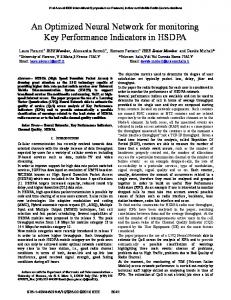
Map showing Lake Okeechobee, Florida, and location of numbered inflow and outflow points.............................. 3 Diagram showing partitioning of load error into discharge and concentration components...................................... 7 Diagram showing optimization routine and resultant relation of uncertainty to cost.................................................11 Schematic of selection order for optimum benefit-cost improvement in monitoring.................................................12 Hydrograph of inflow and outflow for Lake Okeechobee, water year 1986 ..............................................................14 Maps showing spatial distribution of average phosphorus concentrations, discharge, computed phosphorus loads, and standard load errors for Lake Okeechobee, 1982-91 ............................................16 7-9. Plots showing: 7. Relation of phosphorus-loading rate to discharge and concentration on five principal tributaries to Lake Okeechobee, 1981-92 ...........................................................................................21 8. Observed phosphorus concentrations and estimates computed from regression of loads for five selected sites ............................................................................................................................22 9. Uncertainty in annual load estimates as a function of increasing monitoring cost in 1992 dollars ............................................................................................................................................26 10. Diagram showing an optimized set of network changes decrease uncertainty in nutrient load estimates for Lake Okeechobee at a cost of $200,000 (1992 dollars) ........................................................................27 Tables 1. Points of discharge and data collection around Lake Okeechobee ......................................................................... 4 2. A hydrologic budget for Lake Okeechobee for water years 1982 to 1991 .............................................................13 3. Mean and standard deviation of phosphorus concentration data for samples collected at selected discharge points around Lake Okeechobee ...............................................................................................17 4. Summary of phosphorus loads for tributaries to Lake Okeechobee .......................................................................18 5. Coefficients for estimation of loads based on regression analysis loading data at major tributaries for the period October 1981 through September 1990 ................................................................. .........20 6. Summary of benefits and costs for selected monitoring scenarios .........................................................................24

Contents

III

IV

Contents

An Optimized Network for Phosphorus Load Monitoring for Lake Okeechobee, Florida By W. Scott Gain

ABSTRACT Phosphorus load data were evaluated for Lake Okeechobee, Florida, for water years 1982 through 1991. Standard errors for load estimates were computed from available phosphorus concentration and daily discharge data. Components of error were associated with uncertainty in concentration and discharge data and were calculated for existing conditions and for 6 alternative loadmonitoring scenarios for each of 48 distinct inflows. Benefit-cost ratios were computed for each alternative monitoring scenario at each site by dividing estimated reductions in load uncertainty by the 5-year average costs of each scenario in 1992 dollars. Absolute and marginal benefitcost ratios were compared in an iterative optimization scheme to determine the most cost-effective combination of discharge and concentration monitoring scenarios for the lake. If the current (1992) discharge-monitoring network around the lake is maintained, the waterquality sampling at each inflow site twice each year is continued, and the nature of loading remains the same, the standard error of computed mean-annual load is estimated at about 98 metric tons per year compared to an absolute loading rate (inflows and outflows) of 530 metric tons per year. This produces a relative uncertainty of nearly 20 percent. The standard error in load can be reduced to about 20 metric tons per year (4 percent) by adopting an optimized set of monitoring alternatives at a cost of an additional $200,000 per year. The final optimized network prescribes

changes to improve both concentration and discharge monitoring. These changes include the addition of intensive sampling with automatic samplers at 11 sites, the initiation of event-based sampling by observers at another 5 sites, the continuation of periodic sampling 12 times per year at 1 site, the installation of acoustic velocity meters to improve discharge gaging at 9 sites, and the improvement of a discharge rating at 1 site. INTRODUCTION Nutrient loading has a direct effect on the trophic state, diversity, and stability of aquatic ecosystems and is a major focus of many ecosystem restoration efforts. Because of the interest in nutrient loading rates for the evaluation of trends and ecological effects, the accuracy and precision of load estimates remain a continuing source of concern. Load monitoring at multiple inflow-outflow points around a lake can present an enormous task and expense for data collection and computation. Various optimized decision-making approaches have been used to increase the efficiency with which information is collected in water-quality monitoring networks (Harmancioglu and Alpasian, 1992). These approaches have most often attempted to maximize information in hydrologic data (measurable changes in water quality) relative to noise. Generally, efforts to optimize load-monitoring networks have focused on minimizing uncertainty to concentration data; network-optimization studies have not considered cost in their optimization schemes. Potential errors in the determination of discharge are often ignored or assumed to be unimportant. Abstract

1

The measure and control of uncertainty in loading estimates is critical to the effective management of the ecological resources. The statistical ability of the monitoring networks to identify differences between sites or trends with time can be expressed as the statistical power of the network. Generally, this power is directly related to the extent to which the observed variation in measured loads can be explained by or attributed to relevant biological or chemical processes. Temporal variation can be explained when it can be predictably related to some time-dependent process or pattern (Box and Jenkins, 1970). Variation that cannot be empirically or theoretically related to some relevant process produces uncertainty in any inference derived from time-series data. The statistical power of the network increases as the ratio of explained to unexplained variation increases. The ratio of explained to unexplained variation in measurement techniques is often expressed in terms of the accuracy and precision of the technique. This characterization can be usefully extended from the evaluation of instrument performance (as is most common) to the performance of an entire methodology. Accuracy, which generally refers to the relative systematic deviation of a measured quantity from its “true” value, can be likened in statistical terms to a measure of relative bias. Precision, which is held to be a measure of the random deviation of a measured quantity in relation to its “average measured” value, can be likened in statistical terms to the coefficient of variation (CV) of a sample distribution. Generally, of the two, accuracy is the more difficult to verify because of the uncertainty in obtaining a “true” value for comparison. Precision is somewhat easier to quantify because of its reliance on an “average measured” value, which can be readily obtained from a sample distribution. This report describes a method to help prioritize load-monitoring effort and to increase the statistical power of the network for Lake Okeechobee, Florida. The uncertainty associated with a suite of monitoring alternatives was evaluated for each of 48 discrete nutrient discharges into the lake in a cooperative effort between the U.S. Geological Survey (USGS) and the South Florida Water Management District (SFWMD). An optimized set of monitoring practices was developed to produce the least uncertainty in total load rates for the least additional effort or cost. 2

Purpose and Scope This report presents an approach for evaluating the components of error in loading rates associated with uncertainty in discharge and concentration data. Benefit-cost ratios are determined for each of seven alternative monitoring scenarios, where benefits are measured in terms of an overall reduction in uncertainty in loading rates. An optimized network for water-quality sampling and discharge gaging is derived to minimize random uncertainty in load estimates for a given level of effort measured in 1992 dollar costs. In contrast to other optimization methods in the literature, the approach presented here optimizes on both discharge and concentration in comparable terms of load for each of several discrete levels of instrumentation and expense. Although temporal covariance in concentration is addressed to a limited extent in this evaluation (by frequency-domain filtering), spatial covariance is not taken into account as a source of uncertainty in loading rates. Spatial covariance is not considered here because the existing models for load computation fail to incorporate spatial terms and are, therefore, insensitive to optimization in the spatial domain. Although loads of various nutrient chemical species might be considered in a similar analysis, this application is limited to total phosphorus data available from the USGS and SFWMD data bases. Network optimization encompasses three operations—first, an evaluation of the explained and unexplained variations in daily mean loading rates based on available data; second, the computation of uncertainty estimates for each of several potential monitoring alternatives; and third, the selection of the most cost-effective combination of monitoring alternatives to produce the greatest overall decrease in uncertainty for the least increase in monitoring expense. Background on Lake Okeechobee Lake Okeechobee is the second largest lake in the coterminous United States and is an important part of the hydrologic system of the Everglades in south Florida. The lake is 675 square miles (mi2) in area and contains about 4 million acre-feet (acre-ft) of water at a typical stage of 15 feet (ft) above mean sea level. Because much of the water flowing through the Everglades originates in or passes through Lake Okeechobee, the trophic status of the lake and the rates


of nutrient loading in surface-water discharges from surrounding basins have become the focus of public attention. Consequently, a loading target has been established for the lake as part of Florida law (Storm Water Management Model (SWMM), 1992). To meet this target, maximum permitted nutrient-loading rates have been established by SFWMD for each of numerous tributaries to the lake. The size of the lake and the complexity of hydrologic inputs and outputs make a comprehensive evaluation of nutrient loads for the entire lake difficult and expensive. Surface-water drainage can enter or leave the lake through any of 48 distinct sources (fig. 1, table 1). Most of these are controlled by structures at the lakeward end of a complex system of canals that are used alternately to provide irrigation or drainage depending on the weather and season. Only discharge to the lake from the west through Fisheating Creek remains uncontrolled. Backpumping of drainage water from agricultural land can significantly increase the concentrations of nutrients in

a rim canal around the lake from which water may enter the lake in small quantities at any of numerous locations. Concentrations of phosphorus in backpumped water may be high in some agricultural discharges, but concentrations are not consistently high throughout the basin and vary substantially with season (Dickson and others, 1978). The SFWMD computes daily and annual loads for each of the 32 larger sources of nutrient inflow (SWMM, 1992). Inflows into Lake Okeechobee may be divided into nine subbasins (table 1). These subbasins are hydrologic units that tend to have similar discharge characteristics and within which drainage systems are often hydraulically connected through a series of linking canals. This is particularly true in subbasins 7, 8, and 9 where agricultural ditching has completely altered the natural drainage. Because of the connectivity within subbasins, the sizes of contributing areas and area-based yields are difficult to determine. As a result, precise load estimates require discharge and concentration data for all major discharges to the lake.

Taylor Creek

Ki ssi mm Ri ee ve r

441

Nubbin Slough

STUDY AREA

Okeechobee 13 9 12 11 dia nP 14 Ca ra 10 8 7 6 54 3 Ha n i r a ie rn l 15 e 2 Ca y P o 18 na nd 78 16 l 17 In

27

22 20 21 24 Fisheating Creek

23

Lake Okeechobee

25 26 28

80

29

30 31 32

41 33

27

34

Clewiston

35 36

48 47 46 45 44 43 42 Wes tP alm

40 441 39 38 Belle Glade 37

Induscan Canal

Miami Canal

Figure 1.

ie C Luc St.

19

27 Caloosahatchee River

EVERGLADES

1

L-

8C

l ana

an al

Be ac hC an al

N 0 0

5 5

10 MILES 10 KILOMETERS

Hillsboro Canal North New River

Lake Okeechobee, Florida, and location of numbered inflow and outflow points.

Introduction

3

4

Table 1. Points of discharge and data collection around Lake Okeechobee

An Optimized Network for Phosphorus Load Monitoring for Lake kOkeechobee, Florida

[HGS, Hurricane Gate Structure; ft3/s, cubic feet per second; Do., ditto. Discharge rating: T, theoretical; M, measured; **, no rating. Discharge record: L, log; R, recorder; U, ungaged. Water quality analysis: I, inorganic constituents; N, nutrients. Water quality agency: SFWMD, South Florida Water Management District; USACE, U.S. Army Corps of Engineers; USGS, U.S. Geological Survey] Subbasin

1

2

3

4

5

Site number

1 2

USGS site number

02275705

3 4 5 6 7 8

02275606

9 10 11 12 13 14

02273000

15 16 17 18 19 20 21 22 23 24 25

6

26 27

7

28 29 30 31 32 33

02275503

02273300

02259200

02257800

02257000

02292001

Site name

Discharge

Latitude/ longitude

Type of control 3

Rating

Water quality

Record

Agency

Analysis

Agency

S-135 Henry Creek Lock (HCL)

270510 0803941 270943 0804304

4-125 ft /s pumps, 15’ lock, 2-10’ lift gates 15’ lock

T M

L R

SFWMD USGS

N, I

SFWMD Do.

S-191 on Nubbin Slough C-9 C-8 S-133 on Taylor Creek HGS-6 C-7

271136 0804545 271149 0804619 271207 0804649 271224 0804753 271224 0804753 271220 0804805

4-27’ lift gates 3 flap gates on 3-10’ culverts 3 flap gates on 3-10’ culverts 5-125 ft3/s pumps, 30’ lock 30’ lock 3 flap gates on 3-10' culverts

T T T M M T

L L L R R L

SFWMD USACE USACE USGS USGS USACE

N, I

SFWMD Do. Do. Do. Do. Do.

S-65E on Kissimmee River C-6 C-38W S-154 and S-154C S-84 on C-41A L-59E

271332 0805746 270951 0805254 271159 0805436 271241 0805506 271255 0805855 271130 0805412

6-27' lift gates, 30' lock 1 lift gate on 1-10' culvert 1 lift gate on 1-10' culvert 2-10' lift gates 2-27' lift gates 1 flap gate on 1-10' culvert

M T T T M T

R L L L R L

USGS USACE USACE SFWMD SFWMD USACE

N, I

N, I N, I N, I

USGS, SFWMD Do. Do. SFWMD USGS, SFWMD SFWMD

S-127 at Buckhead Lock L-59W at S-72 L-60E at S-72 L-60W at S-71 S-72 on Indian Prairie Canal S-129 L-61E at S-71 S-71 on Harney Pond Canal S-131 at Fisheating Lock

270719 0805346 270533 0810023 270533 0810027 270157 0810413 270535 0810025 270147 0810006 270157 0810417 270200 081045 265842 0810524

5-125 ft3/s pumps, 15' lock, 1-10' lift gate 2 flap gates on 2-10' culverts 2 flap gates on 2-10' culverts 2 flap gates on 2-10' culverts 2-27' lift gates, 1-125 ft3/s pump 3-120 ft3/s pumps, 1-10' lift gate 2 flap gates on 2-10' culverts 3-27' lift gates, 1-125 ft3/s pump 2-120 ft3/s pumps, 15' lock, 1-10' lift gate

T T T T M T T M T

L L L L R L L R L

SFWMD USACE USACE USACE SFWMD SFWMD USACE SFWMD SFWMD

N, I N, I N, I N, I N, I N, I N, I N, I N, I

SFWMD Do. Do. Do. USGS, SFWMD SFWMD Do. USGS, SFWMD SFWMD

L-61W at Hoover Dyke Fisheating Creek (FEC) at SR-78

265806 0810811 265744 0810715

2-10' flap gates no structure-lake level control outflow

T **

L U

USACE USGS

N, I N, I

SFWMD Do.

C-5 C-5A

265508 0810722 265305 0810722

3 flap gates on 3-10' culverts 2 flap gates, 1 lift gate on 3-10' culverts

T T

L L

USACE USACE

N, I

SFWMD Do.

S-77 on Caloosahatchee River

265020 0810508

4-27' lift gates, 30' lock

M

R

USGS

N, I

SFWMD

C-1 C-1A S-4 C-2 S-310 and HGS-2 on Induscan Canal

264938 0810356 264855 0810035 264722 0805743 264725 0805747 264514 0805508

2 flap gates on 2-10' culverts 3 flap gates on 3-10' culverts 3-860 ft3/s pumps 5 flap gates, 1 lift gate on 6-10' culverts 30' lock

T T T T **

L L L L U

USACE USACE SFWMD USACE SFWMD

N, I

Do. Do. Do. Do. Do.

N, I N, I,

N, I

Table 1. Points of discharge and data collection around Lake Okeechobee [HGS, Hurricane Gate Structure; ft3/s, cubic feet per second; Do., ditto. Discharge rating: T, theoretical; M, measured; **, no rating. Discharge record: L, log; R, recorder; U, ungaged. Water quality analysis: I, inorganic constituents; N, nutrients. Water quality agency: SFWMD, South Florida Water Management District; USACE, U.S. Army Corps of Engineers; USGS, U.S. Geological Survey] Subbasin

8

Site number

34 35 36 37 38

USGS site number

02286400 02280000

39 40 41 9

42 43 44 45 46 47 48

02278000

02276870

Site name

Latitude/ longitude

Discharge Type of control

Rating

Water quality

Record

Agency

Analysis

Agency

S-236 C-3 S-3 and HGS-3 on Miami Canal C-4A S-2 and HGS-4 on North New River C-12 C-12A C-10

264340 0805111 264315 0805030 264155 0804825 264056 0804502 264200 0804300

3-85 ft3/s pumps 1 flap gate, 1 lift gate on 2-10’ culverts 3-860 ft3/s pumps, 2-27’ lift gates 1 flap gate on 10’ culvert, private pump 4-900 ft3/s pumps, 3-27’ lift gates

T T M T M

L L R L R

SFWMD USACE USGS USACE USGS

N, I N, I N, I

SFWMD Do. Do. Do. Do.

264455 0804105 264634 0804137 264753 0804146

2 flap gates, 1 lift gate on 3-10’ culverts, 1 flap gate on 1-7’ culvert, private pump 1 flap gate, 1 lift gate on 2-10’ culverts

T T T

L L L

USACE USACE USACE

N, I N, I N, I

Do. Do. Do.

S-352 and HGS-5 on West Palm Beach Canal C-13 C-10A on L-8 Canal C-14 C-16 C-11 S-308B and S-308C on St. Lucie Canal

265150 0803755

2-27’ lift gates

M

R

USGS

N, I

SFWMD

265359 0803644 265501 0803649 265635 0803641 265709 0803641 265756 0803644 265900 0803700

1 lift gate on 1-10’ culvert 4 flap gates, 1 lift gate on 5-10’ culverts 1 lift gate on 1-10’ culvert 1 lift gate on 1-10’ culvert 1 lift gate on 1-10’ culvert, private pump 4-27’ lift gates, 30’ lock

T M T T T M

L R L L L R

USACE USGS USACE USACE USACE USGS

N, I

N, I

N, I

Do. Do. Do. Do. Do. Do.

Introduction 5

Phosphorus management goals are outlined by the SFWMD in the Lake Okeechobee SWMM Plan which sets forth target performance standards for inflow phosphorus concentrations for each of the 32 monitored inflows within the district. The target standards were established to produce in-lake phosphorus concentrations below the eutrophic range indicated by a modification of the Vollenweider model. The concentration target for each inflow is set at the lesser of an annual flow-weighted concentration of 0.18 milligram per liter (mg/L) or the flow-weighted average of historical data. When the flow-weighted concentration target of 0.18 mg/L or less is met consistently at all inflows, the overall target phosphorus load of 397 tons per year for the lake also should be met (SWMM, 1992). Phosphorus concentrations and surface-water discharges are monitored at each of the 32 inflow and outflow sites around the lake. Discharges are monitored continuously and concentrations are sampled on 2- to 4-week intervals. From these data, daily and annual loading estimates and flow-weighted concentrations are computed. Discharge at many of the monitoring points is intermittent and samples are periodic. The natural variability in both the discharge and concentration data presents problems in comparing daily and long-term loading rates to SWMM standards. Loading estimates for Lake Okeechobee generally have been computed using a time-weighted average interpolation method to determine concentration. Daily mean nutrient concentrations have been interpolated from periodic sample data (typically biweekly). These interpolated concentrations are then multiplied by gaged discharges to compute a daily load which is averaged for a given period. Automatic samplers have been used to increase sample frequency at some sites, but samplers can be costly to operate and have not been employed throughout the monitoring network. The computed average loads incorporate the variability associated with the sample concentration data and daily discharge. The effects of natural variability on computations of overall lake-loading rates have not previously been taken into account in evaluations of temporal trends and compliance with loading standards.

APPROACH AND METHODOLOGY Network-monitoring optimization presented here is based on: (1) an evaluation of uncertainty in computed loads due to variability and uncertainty in both discharge and concentration data, and (2) an evaluation of potential changes in uncertainty in these data 6

given each of several selected monitoring alternatives employed at each of the 48 flow points identified around the lake. Benefit-cost ratios computed for each monitoring alternative at each network site can then be compared and the most cost-effective set of monitoring alternatives for all sites can be selected. Because variations due to measurement and natural variability are cumulative, the uncertainties described in this report refer to a composite of measurement and sampling (representation) errors. Daily discharge data for many tributaries were obtained from the USGS data base and were computed using standard USGS methods (Rantz and others, 1982). Discharge data at several other structures were obtained from the SFWMD data base and were computed from operator records at several hydraulic structures and theoretical structural ratings. Daily discharges for many of the smaller inflow points were estimated by comparison to adjacent sites. Evaluation of Uncertainty Tributary loading may be viewed as the integrated product of two time series, one consisting of sequential observations of discharge and the other of sequential observations of concentration. Within each of these time series, the observed value is an approximation of the true, or expected, value at any point in time. Differences between measured and expected time series may result from both systematic and random errors (a combination of measurement and sampling errors). Systematic differences, or biases, are difficult to identify and measure but can be reduced by rigorous quality-assurance standards. Random errors tend to increase the observed random variability in calculated loads but can be reduced by averaging. The aggregate uncertainty in loads due to random processes can be estimated from the observed variability of discharge and concentration data after an estimate of expected variation has been subtracted. The standard approach to computing the load time series is given by equation 1: Lt = Ct × Qt ,

(1)

where C t is measured concentration at time t, Q t is measured discharge at time t, L t is a computed load based on measured values of concentration ( C t ) and discharge ( Q t ).


Assuming random errors in estimating the expected values of discharge and concentration (errors are independent of any covariance in C t and Q t ), measured values can be related to expected values by equations 2 and 3: Ct = ct + ec , t

(2)

Qt = qt + eq , t

(3)

where c t is expected concentration at time t, q t is expected discharge at time t, e c is random error in the measurement of (c) at t time t, and e q is random error in the measurement of (q) at t time t. The error terms e ct and e q t can generally be assumed to be independent and random in Q and C time series so by substitution of equations 2 and 3 into equation 1, and the expression for measured load becomes: Lt =  ct + ec   qt + eq  ,  t  t

(4)

which can be factored to an expression of expected load:

qc t = L t –  ce q + qe c + e q e c  ,  t t t t

(5)

where qc is the expected load at time t, ceq is the partial error in L t associated with e q t at time t, qec is the partial error of L t associated with e c t at time t, and eqec is the product of errors in Q t and C t at time t. Equation 5 explains the partitioning of uncertainty in load estimates into partial products. This also is illustrated by the square in figure 2. The partial error associated with uncertainty in concentration (concentration load error) and the error associated with uncertainty in discharge (discharge load error) are independent and random. Even where the expected values of discharge and concentration are covariant, the random errors in these terms are independent. The product of errors (eq ec) varies in proportion to discharge and concentration load errors, but tends to be small for coefficients of variation less than 1. Given that errors in ec and eq are assumed to be independent, the standard error of measured loads can be approximated by the joint probability of partial error terms expressed in equation 5 by substituting standardized errors (sc and sq) for discrete errors ( e ct and e q ) in each partial error term, and estimating t expected values from the mean of measured values.

Load error associated with discharge error Load error associated with the interaction of discharge and concentration error eQ

+ -

eQ eC

C e Q

Load Q

Q C

Q eC

Load error associated with concentration error -+

C

eC

C Q eC eQ

is measured concentration is measured discharge is error in measured concentration is error in measured discharge

Figure 2. Partitioning of load error into discharge and concentration components—load is represented in the area formed by the product of discharge and concentration, errors in load are represented by shaded rectangles. Approach and Methodology

7

The joint probability of summed errors can then be estimated as: sL =

2 2 2 ( Q × sc ) + ( C × sq ) + ( sc × sq )

,

(6)

where sL is the estimated standard error of measured loads, sq is the standard error of measured discharge, sc is the standard error of measured concentration, Q is average measured discharge, and C is average measured concentration. This simplification ignores the errors in estimating the expected values of q and c by Q and C ; however, these errors are assumed to be small for large sample sizes. Standard errors sq and sc are determined as the average difference between each measured value and the mean of all measurements (the estimated expected value). When the expected value of a time series is stationary, the random uncertainty can be estimated as the standard deviation of the observed data set. However, when a time series varies with some expected frequency, periodic variation is included in the measured deviation of the time series. As a result, the standard deviation of the time series overestimates actual random uncertainty. To improve estimates of uncertainty, estimates of s c and s q were refined by indentifying and removing periodic variation in the expected time series. Continuous time series of Q and C are not actually measured at the temporal scale needed for load estimation. Instead, models are used to interpolate from observations of Q and C, based on the observed or assumed behavior of the expected time series q and c. As a class, models include any implied or explicit assumptions made about the behavior of q and c— including assumptions about simple straight-line relationships between successive observations. Conceptual models are then calibrated against periodic measurements Q and C. Standard errors of estimates ( s qˆ and s cˆ ) for the modeled time series can be computed as the average squared difference between periodic observations and model predictions at a given time. This provides a composite measure of error associated with both the modeling and the measurement of q and c. The classic model for the computation of q, applied within the USGS, is the shifting-control method and rating-curve approach (Rantz and others, 1982). 8

This approach can be extended somewhat to include structural ratings at hydraulic control structures. In either case, the discharge rating provides an estimate of the behavior of q over time against which measurements of Q are compared and an estimate of s qˆ derived. Random errors in estimated q, based on continuous record of stage, are due to random, transient changes in streamflow hydraulics in natural channels and at hydrologic control structures, and attributed to channel scour and deposition and the accumulation of debris. The history of discharge measurements at sites around Lake Okeechobee and at sites on other lowgradient streams in Florida gives an indication of the random error in discharge models. Discharge measurements generally are rated in accuracy between 5 and 10 percent but may deviate from a given discharge rating by as much as 30 percent. Some of the measurement deviation from ratings can be attributed to systematic changes or shifts in control conditions, which are predictable and are corrected in discharge computations. However, the extent of measurement deviations from rating that is caused by random uncertainties can be substantial in terms of total discharge. This uncertainty typically is estimated to be as much as 20 percent. Models for predicting cˆ are not as well established as those for discharge; no single model has gained complete acceptance. The SFWMD has adopted a linear-interpolation model for computing loads to Lake Okeechobee. This model is only one of several possible alternatives and may be no better or worse than others. However, the interpolation model without modification is over parameterized and lacks the necessary degrees of freedom to evaluate s cˆ . For the purposes of this analysis, a linear-regression model was used to predict c for all major tributaries except those for which reliable estimates of q were unavailable. Average concentrations for remaining discharge points were computed from available concentration data. Concentration models were developed for each major tributary to Lake Okeechobee based on the following relation in which load ˆl is obtained using leastsquares regression in the following general form:


ˆl cˆ = --qˆ ,

(7)

and

ˆl = 10

2  σ L  β + β Log qˆ + β T + β D + β S + … + β - 1 10 2 3 4 1 n + 3 S n + ----- 0 2  

where ˆl β qˆ T D S

is modeled estimate of expected load, is a linear coefficient, is estimated daily mean discharge, is cumulative time, is the flow direction, is a seasonal term composed of sine and cosine terms, and σ is the standard error of regression. In linear form, ˆl and qˆ are expressed in log units. The data are log-transformed to remove the tendency toward increasing variance with increasing discharge. Log-transformation bias is corrected by the addition of 1/2 of the variance of the load. This corrected value provides a minimum-variance unbiased estimator (MVUE) of the mean phosphorus load (Gilbert, 1987). Multiple seasonal terms can be added to account for variations in expected concentration for periods less than or greater than 1 year. Load-estimation models can be grouped into several general types (Preston and others, 1989), including averaging estimators, ratio estimators, and regression estimators. The accuracy and precision of each of these types depends to a large extent on the population distribution of the data. Although one estimation method may produce unbiased estimates of nutrient load, those estimates may be of such large variance that they are of little practical value; other estimates of greater precision may be biased. The regression method was confirmed by Preston and others (1989) to be a robust and precise method. It has been applied with modification in several loadmodeling studies and has been used as a linear filter technique for trend analysis (Hirsch and others, 1992). The standard error of estimated concentration ( s cˆ ) is directly proportional to the standard error of ˆl from equation 8. The general equation from Neter and Wasserman (1974) explains that the standard error of a linear model is determined by the standard error of the regression, the number of observations included in the regression analysis, and the difference between the

S

l TOTAL

=

considered value of the independent variable for a given estimate and the mean of the independent variable included in the regression analysis.

s

Yˆ

(X – X) 1 = SER --- + ------------------------n 2 Σ( X – X)

.

(9)

Equation 9 reduces to the standard error of the mean of regression residuals at the mean of the independent variable (X). Substituting the estimated load ( ˆl ) for Y and discharge ( qˆ ) for X in equation 9, the standard error of the mean load estimate at a mean discharge becomes: SER s = ----------- , ˆl n

(10)

the standard error of estimated concentration is then: sˆ (11) s c = ---l , q and is strictly proportional to the standard error of the mean of loads in equation 10. Network Optimization The network was optimized by minimizing the random and systematic errors in total load estimates for a given level of monetary investment. The goal of optimization was to produce the most cost-effective reduction in discharge-load and concentration-load errors by determining at which sites and for which instrumentation and sampling methods the greatest reduction in overall load error could be expected. This is achieved conceptually by minimizing equation 6, after summing for all sites and normalizing for cost. Equation 12 represents the summation of partial error terms for all 48 sites:

2 2 2 48  c × s  s × s  q ×s   i c  i q  c  i i i qi --------------------------- + --------------------------- + ----------------------------f f f ×f ci qi ci qi i=1

∑

(8)

,

Approach and Methodology

(12)

9

where s c is the standard error of mean c at site i for a i given period of time, s q is the standard error of mean q at site i for a i given period of time, f is the dollar cost of the alternative, and i is an index of inflow point. Squared error terms are divided by costs ( f c ) to obtain a measure of variance per unit cost. These terms are then summed to obtain the overall weighted variance per unit cost. The goal of optimization as expressed in equation 12 is to identify sampling and monitoring practices that produce the greatest possible reduction in variance for a given cost, where the sum of costs is limited by management prerogatives (eq. 13): n

∑  fci + fqi = COSTLIMIT

. (13)

i=1

Because the monitoring alternatives considered in this analysis represent discrete levels of effort, standard errors for each monitoring alternative are discontinuous (stepping). This precludes the solution of equation 12 by standard linear or nonlinear techniques. As an alternative approach, a discrete solution utilizing an iterative selection process was developed. Various feasible monitoring alternatives to the current flow- and concentration-sampling network were identified. These alternatives included a range of options for both discharge and concentration. Sampling costs and benefits for each alternative were then evaluated for each of the 48 sites around the lake. The Orlando Subdistrict of the USGS averaged 5-year costs (in 1992 dollars) for installation and operation of standard stream-gaging and water-quality sampling equipment. Benefits were determined as a difference in the squared mean standard errors of partial error terms summed as in equation 6. By partitioning the loading error into partial terms involving discharge and concentration (partial products involving q i and c i in eq. 12), we directly compared costs and benefits of possible modifications to the discharge-monitoring network with the costs and benefits of possible alternatives to the concentration-monitoring network. Standard errors of discharge were determined from experience with various measurement and gaging techniques of the USGS and the observed success of various techniques in low10

velocity streams in Florida (Sloat and Gain, 1995). Partial standard errors from concentration were calculated as in equations 9 and 10 and based on an expected replication factor (n) determined for each sampling alternative for a given sample period. A sample period of 1 year was assumed—based on the need for annual load estimates. Benefit-cost ratios were computed for marginal differences between all monitoring alternatives for each site and for both concentration and discharge monitoring alternatives. An optimized set of network enhancements was selected from among various monitoring alternatives by use of a manual, iterative selection process similar in nature to dynamic programming. The selection algorithm is illustrated in figure 3 and comprises the following steps: (1) rank marginal benefit-cost ratios for all sites and monitoring alternatives comparing each alternative to the existing baseline condition (the baseline may be an existing practice at a given site or any assumed minimal level of monitoring), (2) identify the maximum ratio and substitute the alternative for the baseline condition at that site, (3) re-rank benefit-cost ratios comparing baseline and possible alternatives and incorporate the new baseline substituted in the previous step, (4) identify the maximum marginal benefit-cost ratio and again substitute the alternative for the baseline, and (5) sum the total cost of monitoring. This selection process is repeated in the same manner until a predetermined cost limit is reached. Ultimately, the cost limit is affected by optimization and may be based on the marginal benefit of loading information relative to other management initiatives. The schematic in figure 3 is simplified to show only two sites and three alternatives; however, the process is the same regardless of the number of sites and alternatives. The slopes of line segments in figure 3 represent benefit-cost ratios. By sequentially selecting the line segments of greatest slope (greatest marginal benefit-cost ratio), the resultant curve will have the most rapid increase in overall benefit for a given increase in total cost. The inverse of this curve (fig. 3) indicates the most rapid decrease in error for a given increase in cost. The example in figure 4 illustrates the process of selection in tabular form. Numbered selections indicate the order in which a given site and monitoring alternative is implemented. Selection starts with the highest benefit/cost ratio of 43.4 and continues to a low of 0.72. After the initial selection of alternative 2


OPTIMIZATION ALGORITHM

Benefit

Benefit

Monitoring alternatives 2 Sites A 1

Baseline condition

2 A

Cost

Cost

1. Evaluate marginal benefit-cost ratios for all monitoring alternatives 2. Select alternative A for Site 1 (greatest marginal ratio as indicated by the slope of the line)

UNCERTAINTY IN ESTIMATE

Sites

1

3. Re-evaluate marginal benefit-cost ratios excluding initial alternative for Site 1 4. Select alternative A for Site 2

Idealized curve showing optimized data collection -- produces most rapid decrease in uncertainty for increasing cost Curve showing unoptimized data collection

COST

Figure 3. Optimization routine and resultant relation of uncertainty to cost.

on site C, the process continues with the implementation of 10 other monitoring alternatives on other sites until the highest remaining benefit-cost ratio is the marginal ratio of alternative 3 compared to the new baseline alternative 2 on site C (2.26 benefit /cost ratio). At this point, monitoring on site C is upgraded from alternative 2 to 3 (shown by the shaded arrow in fig. 4) as is monitoring on 4 subsequent sites (I, J, M, and Q) upgraded to more costly monitoring alternatives. The benefit/cost ratios computed are limited to marginal differences between mutually exclusive alternatives (i.e., sampling 12 times per year compared to sampling only twice per year). Marginal benefitcost ratios are not computed for alternatives 1 and 2 because these alternatives are not mutually exclusive (as, for instance, discharge monitoring and concentration sampling can both be implemented concurrently). As previously noted, the final limitation on this process is cost. Ultimately, with unlimited cost, the

most expensive alternatives will be selected on all sites so long as these alternatives produce some marginal reduction in error. The object of this procedure is not to minimize the error in load estimates, but to maximize the rate of reduction so as to achieve the greatest possible reduction in error for some minimum desirable cost.

RESULTS AND DISCUSSION Discharge A summary of average annual discharge in and out of Lake Okeechobee for the period 1982-91 shows the sources of inflow and the potential magnitude of errors (table 2). Atmospheric fluxes were adopted from James and others (1995) for a 20-year period Results and Discussion

11

BENEFIT-COST RATIOS

Structure Name

Alternative No. 1

Alternative No. 2

Alternative No. 3Alternative No. 2, Marginal BenefitCost Ratio

Alternative No. 3

Site A

0.0

0.0

0.44

Site B

0.02

0.1

0.02

0.31 0.04

Site C

0.36

1

43.4

12 2.26

14.01

0.1

0.16

0.87

9

3.0

0.16

1.71

0.1

Site D

0.57

Site E

0.17

Site F

0.0

0.02

0.05

Site G

0.06

16

1.2

0.23

0.53

Site H

0.01

0.12

0.62

Site I

0.36

14 1.79

4.23

Site J

0.40

13 1.8 6 10.1 3 15.3

15 1.44

5.55

Site K

0.01

0.1

0.01

0.05

Site L

18 0.82

0.3

0.01

0.10

Site M

0.14

5

14.4

0.0

10

2.5

17 0.86 0.19

4.78

Site N Site O

0.39

7

6.2

0.53

2.18

Site P

0.08

4

14.9

4.84

Site Q

0.0

0.1

19 0.72 0.03

Site R

0.08

2

28.3

0.65

8.70

Site S

0.05

11

2.3

0.42

0.96

Site T

0.038

8

4.8

0.604

1.83

0.86

0.04

Figure 4. Schematic of selection order for optimum benefit-cost improvement in monitoring— numbered boxes indicate the order in which an alternative on a particular site is selected for implementation based on a comparison of relative and marginal benefit-cost ratios.

from 1973 to 1992. This hydrologic budget is similar to that reported by Joyner (1974) and Maddy (1978) and the surface-water fluxes are similar to those reported by James and others (1995). Lake evapotranspiration estimates also are similar to a previous regional estimate by Farnsworth and others (1982). From 1982 to 1991, inflow to the lake averaged 4,380 cubic feet per second (ft3/s). Of this, more than onethird (about 1,710 ft3/s) is derived from rainfall alone. Of the 4,550 ft3/s of outflow, evaporation comprised the largest single sink (2,800 ft3/s), followed by surface-water discharge (1,480 ft3/s) flowing largely through three structures: S-77, on the Caloosahatchee River to the southwest; S-308, on the St. Lucie Canal to the east; and S-2, flowing south through the Hillsboro Canal to the Everglades agricultural area. The intra-annual distribution of daily mean surface-water discharges within the year is driven by a combination of stormwater runoff and agricultural withdrawal and releases (fig. 5), and the daily balance of inflows and outflows varies seasonally. In the 12

example shown in figure 5 (water year 1986), daily discharges entering the lake range from 0 to more than 8,000 ft3/s and daily discharges leaving the lake range from near 0 to more than 4,000 ft3/s. During periods of high rainfall, inflow to the lake is increased by both surface-water runoff upstream and the return of water from inundated agricultural land, or backpumping. Backpumping from agricultural land usually is greatest from May through September (Dickson and others, 1978). Large releases from the lake are usually made in April and May to increase the flood-control capacity of the lake before the wet season of July through September. Estimated standard errors in discharge (table 2) reflect an average error for gaged inflows of about 20 percent but vary by site according to the demonstrated reliability of the existing data at each site. The total error for all inflows (given the joint probability of errors) reduces to about 5 percent. Annual discharge data using standard gaging practices typically are considered to be accurate only to within a range of about


Table 2. A hydrologic budget for Lake Okeechobee for water years 1982 to 1991 [--, no data; HGS, Hurricane Gate Structure; ft3/s, cubic feet per second]

Subbasin

Site name

Source

Outflow (ft3/s)

Outflow estimated standard error (ft3/s)

--

--

--

--

3 29

---

---

1,230 169 52

180 25 25

----

----

Gaged Gaged Gaged Gaged Gaged Estimated

22 35 14 222 6 8

5 5 2 44 1 4

-------

-------

FEC L-61W

Gaged Estimated

246 2

40 2

---

---

6

C-5, C-5A

Estimated

30

7

--

--

7

S-77 S-4 C-1, C-1A, C-2, S-310, HGS-2

Gaged Gaged Estimated

13 26 --

5 3 --

467 -53

70 -25

8

S-236 S-3, HGS-3 C- 4A S-2, HGS-4 C-12 C-12A C-10 C-3

Gaged Gaged Gaged Gaged Gaged Gaged Gaged Estimated

5 51 8 98 10 11 7 3

1 7 1 15 1 1 3 2

-180

-31 -48 -----

S-352, HGS-5 C-10A S-308B, S-308C C-13, C-14, C-16, C-11

Gaged Gaged Gaged Estimated Gaged

3 68 134 12

2 10 40 6

82 57 326 --

2,429 241

196 39

1,432 53

1,712

86

2,806 262

140 --

4,382

217

4,553 171

195

1

S-135 HCL

2

Gaged

Inflow (ft3/s)

Inflow estimated standard error (ft3/s)

Estimated

23 3

2 2

S-133 S-191, C-9, C-8, HGS-6, C-7

Gaged Estimated

28 131

3

S-65E S-84 C-6, C-38W, S-154, S-154C, L-59E

Gaged Gaged Estimated

4

S-127 S-72 S-129 S-71 S-131 L-59W, L-60E, L-60W, L-61E

5

9

All

Surface water

Estimated Atmospheric Change in storage (4 ft) Total Residual (Inflow-outflow)

320 -----

14 9 98 -134 25

Results and Discussion

13

10,000

INFLOW AND OUTFLOW, IN CUBIC FEET PER SECOND

8,000 6,000

MEAN DAILY INFLOW (1,850 ft3/s)

DAILY MEAN INFLOW

4,000 2,000 0 -2,000 -4,000

MEAN DAILY OUTFLOW (-600 ft3/s)

DAILY MEAN OUTFLOW

-6,000 O

N

D

J

F

1985

M

A

M

J

J

A

S

1986

Figure 5. Hydrograph of inflow and outflow for Lake Okeechobee, water year 1986.

5 to15 percent based on the accuracy of individual discharge measurements (within about 5-8 percent) and the magnitude of stage-shift corrections in lowgradient streams (typically 5-20 percent). The standard error of budget residuals reported in James and others (1995) for the period 1982 to 1991 was 255 ft3/s. When assuming equal errors in the measurement of inflow and outflow, the standard error of each component can be estimated as the square root of one-half the squared standard error of the budget residuals. From the data of James and others (1995), this amounts to about 180 ft3/s for total inflow and total outflow, which is similar to the standard errors reported for inflow (217 ft3/s) and outflow (195 ft3/s) in table 2. An average annual flux into lake storage of +260 ft3/s occurred during 1982 to 1991; subtraction of outflow from inflow indicates a net overage in outflows of about 170 ft3/s. Meyer (1971) estimated that about 22 ft3/s of the outflow may be accounted for by levee seepage into the lake. The remaining residual hydrologic flux may represent an accumulation of errors in unmeasured sources or poorly measured sinks over the period of study. The annual water budget from James and others (1995) shows a similar overage in outflow (190 ft3/s). Although the magnitude of this budget residual is relatively small compared to total inflow and outflow (only about 14

4 percent), it is notable that the overage is about equal to the combined inflow from all but the twelve largest tributaries to the lake (204 ft3/s). The greatest part of the random error in hydrologic budgets can be attributed to errors in the measurement and estimation of surface-water discharge. Though rainfall is spatially and temporally variable, rainfall is spatially diffuse and can be measured accurately and independently at numerous random locations with relatively little bias. Evaporation from the surface of a lake—though subject to bias, particularly where measured in pans (Winter, 1981)— is spatially uniform and temporally predictable. A similar point can be made for ground-water seepage for which changes in hydrostatic head over time are relatively small. Furthermore, though small changes in lake stage equate to large differences in equivalent discharge, changes in lake storage can be measured very precisely—especially when accumulated over a 10year period. Phosphorus Concentrations and Loads Phosphorus-concentration data collected by the USGS in periodic samples from the Kissimmee River (S-65E), Fisheating Creek (FEC), and Harney Pond Canal (S-71), during the period 1982 to 1991,


were compared to SFWMD data from these streams for the same period and differed by only 0.01 mg/L on average. This was not statistically significant so the USGS sample data are used in combination with SFWMD data from these streams and 31 other flowcontrol points around the lake. Although the Kissimmee River is disproportionately the largest source of discharge to Lake Okeechobee, loads are more evenly distributed around the lake because of the spatial variability of phosphorus concentrations (fig. 6). Standard errors of regression represent the magnitude of uncertainty in instantaneous loading estimates due to uncertainties in the concentration model. The standard error of regression is greatest for the Kissimmee River (85 metric tons per year (tons/yr)), although this is not strictly in proportion to discharge. For example, discharge from the Kissimmee River is four times that of the combined inflow and outflow of the North New River (S-2 and HGS-4) on the south side of the lake. The standard error of regression, in contrast, is only about 60 percent larger for the Kissimmee River compared to that of the North New River. Total-phosphorus concentration data for major inflow sites are separated by flow direction into three categories: no-flow, inflow, and outflow (table 3). Samples are identified as no-flow if they were collected on days for which a net discharge of 0.0 ft3/s was computed. Net daily discharges were not determined for all sites. The large proportion of no-flow samples indicated at some sites reflects the episodic temporal distribution of discharge around the lake and the difficulty inherent in periodic sampling schemes in which samples are collected according to a schedule rather than hydrologic conditions. Although most of the differences in concentration with respect to flow direction are small in absolute terms, phosphorus concentrations were marginally higher in flow samples than in no-flow samples at 8 out of 12 inflow sites for which net flows were determined. Notable exceptions to this are average phosphorus concentrations in Fisheating Creek (FEC) and Fisheating Lock (S-131), and at two inflow-outflow sites—C-10A and S-308B and S-308C (St. Lucie Canal)—where concentrations were greater in no-flow samples. Small differences in mean phosphorus concentrations for no-flow and inflow samples may appear to be insignificant when compared to the standard deviations of the data; however, a difference of only 0.02 mg/L when compared to a mean of 0.08 mg/L can induce a bias in load computations of as much as 25 percent.

The standard deviations of combined phosphorus data over the 10-year period range from 0.03 mg/L at S-135 to 0.73 mg/L at S-154. Standard deviations in proportion to the mean were high, ranging from about 50 to 100 percent. The highest concentrations and largest errors were in estimates for the Nubbin Slough (S-191) and Taylor Creek (S-133) Basins to the north of the lake and east of the Kissimmee River. At 13 of the 30 sites listed in table 3, concentrations equalled or exceeded the 0.18 mg/L threshold established as a management goal for Lake Okeechobee. Without additional definition of expected concentrations and increased refinement of standard errors, uncertainties in concentration data make the detection of trends and evaluation of management effects very difficult. Mean annual loading rates estimated for all streams, entering and leaving Lake Okeechobee, are summarized in table 4. The total load entering the lake from all surface-water discharge for the 10-year period was 404 tons/yr. The greatest single contribution of 103 tons/yr (25 percent) came from Kissimmee River (S-65E); the second largest was 84 tons/yr (20 percent) at Nubbins Slough (S-191). Harney Pond Canal (S-71) and Fisheating Creek (FEC) were next in order of load contribution and together accounted for about as much as the Kissimmee River (S-65E). Load contribution from all the remaining streams comprised only about another 110 tons/yr. The total load leaving the lake was only 129 tons/yr, the greatest part of which leaves through the Caloosahatchee River (S-77) and St. Lucie Canal (S-308B and S-308C). Because of the large atmospheric component in the hydrologic budget, atmospheric deposition is a potentially large source of phosphorus to the lake (Joyner, 1974; Swift and others, 1987; James and others, 1995). Although wet deposition may account for a significant phosphorus load to the system, bulk deposition (wet plus dry) has proven difficult to measure accurately due to persistent problems with sample contamination (Peters and Reese, 1995). James and others (1995) inferred a constant phosphorus concentration of 0.03 mg/L in rainwater based on peat-accretion measurements made for the Everglades Water Conservation Area 2A (Walker, 1993). This concentration, though reasonable as a long-term average, reflects a process of accumulation over such an extremely long period (hundreds of years) that annual estimates of load have little meaning. Atmospheric fluxes were not included in this analysis because of the difficulty in determining an annual atmospheric loading rate with any precision.


15

0.36 1230

0.23 0.13 134 0.19

246 0.16

LAKE OKEECHOBEE

LAKE

326

OKEECHOBEE

0.09 466

0.14

0.35

225

0.05 PHOSPHORUS CONCENTRATION, IN MILLIGRAMS PER LITER

93

98

ANNUAL MEAN DISCHARGE, IN CUBIC FEET PER SECOND

N

Kissimmee River

Kissimmee River

85

46 15 41

33

LAKE

LAKE

OKEECHOBEE

27

OKEECHOBEE

1.8 34

12

29

N.New River 14

52

PHOSPHORUS LOADS, IN METRIC TONS PER YEAR 0 0

STANDARD ERROR IN LOAD ESTIMATES BASED ON ONE SAMPLE, IN METRIC TONS PER YEAR 5 10 MILES 5 10 KILOMETERS

EXPLANATION INFLOW

OUTFLOW

Figure 6. Spatial distribution of average phosphorus concentrations, discharge, computed phosphorus loads, and standard load errors for Lake Okeechobee, 1982-91.

16


Table 3. Mean and standard deviation of phosphorus concentration data for samples collected at selected discharge points around Lake Okeechobee [Concentrations are in milligrams per liter. SD, standard deviation; N, number of samples collected; --, no data; HGS, Hurricane Gate Structure] Phosphorus

Site number

Site name

No-flow samples N

Mean

119

Inflow samples

SD

N

Mean

0.07

0.03

24

--

--

1

S-135

3

S-191 on Nubbin Slough

6

S-133 on Taylor Creek

9

S-65E on Kissimmee River

0

--

12

S-154 and S-154C

--

--

13

S-84 on C-41A

14

L-59E

--

--

--

--

--

15

S-127 at Buckhead Lock

--

--

--

--

16

L-59W at S-72

--

--

--

17

L-60E at S-72

--

--

18

L-60W at S-71

--

--

19

S-72 on Indian Prairie Canal

20

S-129

21

L-61E at S-71

22

S-71 on Harney Pond Canal

23

S-131 at Fisheating Lock

25

-114

.19

58

-.09

Outflow samples SD

N

Mean

All samples

SD

N

Mean

SD

0.09

0.03

0

--

--

143

0.07

0.03

--

--

--

--

--

216

.68

.23

36

.33

.14

0

--

--

150

.22

.12

--

217

.11

.08

0

--

--

217

.11

.08

--

--

--

--

--

181

.79

.73

0

--

--

117

.06

.05

--

--

--

--

40

.25

.17

--

--

--

--

--

163

.26

.16

--

--

--

--

--

--

42

.21

.17

--

--

--

--

--

--

--

42

.17

.13

--

--

--

--

--

--

--

44

.16

.14

.05

.05

--

59

-.06

.04

84

.18

.14

45

.19

.09

0

--

--

129

.18

.12

124

.13

.09

24

.17

.12

0

--

--

148

.13

.09

--

--

--

39

.14

.08

--

--

--

--

--

--


62

.16

.12

88

.20

.15

0

--

--

150

.18

.13

115

.11

.06

19

.11

.05

0

--

--

134

.11

.06

Fisheating Creek (FEC) at SR-78

5

.24

.19

121

.18

.15

0

--

--

126

.18

.15

26

C-5

--

--

--

--

--

--

--

--

--

43

.07

.07

28

S-77 on Caloosahatchee River

0

--

--

0

--

--

148

0.09

0.06

148

.09

.06

31

S-4

--

--

--

--

--

--

--

--

--

122

.19

.20

33

S-310 and HGS-2 on Induscan Canal

--

--

--

--

--

--

--

--

--

51

.27

.29

36

S-3 and HGS-3 on Miami Canal

116

.11

.09

37

C-4A

85

.09

.04

38

S-2 and HGS-4 on North New River

152

.15

.10

39

C-12

--

--

--

--

--

--

--

--

--

65

.13

.08

40

C-12A

--

--

--

--

--

--

--

--

--

109

.24

.16

41

C-10

--

--

--

--

--

--

--

--

--

76

.28

.21

42

S-352 and HGS-5 on West Palm Beach Canal

--

--

56

.14

.06

127

.15

.09

44

C-10A on L-8 Canal

48

S-308B and S-308C on St. Lucie Canal

51 --

.08 --

60

.07 --

.14

49 --

.08

.15 --

79

.12 --

.17

16 --

.10

.05 --

13

.02 --

.08

.03

71

.16

.10

0

7

.16

.22

17

.06

.04

11

.12

.05

35

.10

.10

42

.15

.08

22

.13

.04

75

.15

.06

139

.15

.07

17

Table 4. Summary of phosphorus loads for tributaries to Lake Okeechobee [ft3/s, cubic feet per second; tons/yr, tons per year; mg/L, milligrams per liter; --, no data; ( ), estimated value; HGS, Hurricane Gate Structure} Inflow Phosphorus

Subbasin

1

Site name

S-135 HCL S-133 S-191, C-9, C-8, HGS-6, C-7 S-65E S-84 C-6, C-38W, S-154, S-154C, L-59E S-127 S-72 S-129 S-71 S-131 L-59W, L-60E, L-60W, L-61E FEC L-61W C-5, C-5A S-77 S-4 C-1, C-1A, C-2, S-310, HGS-2 S-236 S-3, HGS-3 C-4A S-2, HGS-4 C-12 C-12A C-10 C-3 S-352, HGS-5 C-10A S-308B, S-308C C-13, C-14, C-16, C-11

2

3

4

5 6 7

8

9

Basin

18

Source

No. of No. of days in no-flow period days

No. of inflow days

Mean annual discharge (ft3/s)

Mean annual load (tons/yr)

22.0 3 27.8 131

1.70 .24 8.81 84

LSR Average LSR Average

3,643 -3,600 --

3,196 -3,129 --

447 -471 --

LSR LSR Average

3,652 3,644 --

450 1,885 --

3,202 1,722 --

Average LSR LSR LSR LSR Average

-3,642 3,643 3,642 3,643 --

-2,561 3,135 1,670 3,356 --

-1,081 474 1,958 287 --

22 70 17.6 221 5.8 8

LSR Average Average LSR Average Average

3,594 --3,642 ---

168 --6 ---

3,426 --49 ---

Average LSR Average LSR Average Average Average Average LSR LSR LSR Average

-3,643 -3,643 ----3,652 3,541 3,652 --

-1,966 -2,034 ----2,536 1,111 1,356 --

-215 -290 ----18 1,269 777 --

LSR

--

--

--

2348

Average Total

---

---

---

322 2670

Loadweighted concentrations (mg/L)

Outflow Phosphorus No. of outflow days

0.087 (.09) .355 .68

-----

.093 .155 .62

5.5 5.47 3.07 45.2 .57 1.2

245 2 30 5.7 26 -5 50.9 8 97.5 10 11 7 3 2.3 61.7 129 12

1230 162 52

Mean annual discharge (ft3/s)

LoadMean weighted annual concenload trations (tons/yr) (mg/L)

-----

-----

-----

-37 --

--2.50 --

--1.11 --

-0.496 --

.28 .088 .195 .230 .110 .17

--34 14 ---

---1.86 -2.49 ---

---.221 -.416 ---

---

40.8 .41 1.9 1.80 4.4 --

.187 .101 .072 .352 .19 --

---3587 ---

----474 --53

.36 6.88 .57 11.9 1.1 2.4 1.6 .7 .20 2.73 15.4 1.4

.08 .151 .08 .136 .12 .24 .25 (.25) .095 .050 .134 .13

-1462 -1319 ----1098 1161 1519 --

270

.129

134 404

.465 .169

103 22.4 28

Degree of freedom

Standard error mean load (units)

18 -32 --

1.046 -1.067 --

204 53 --

1.039 1.067 --

.133 .187

-40 17 82 14 --

-1.060 1.109 1.055 1.093 --

----33.8 --9.0

---.080 -.27

114 --141 ---

1.050 --1.038 ---

--182 --321 -----84.5 -58.4 -326 --

--7.48 --14.5 -----9.76 -6.89 -45.9 --

-.046 -.050 ----.129 .132 .157 --

-59 -83 ----50 21 91 --

-1.068 -1.038 ----1.058 1.082 1.040 --

--

1453

120

.092

--

--

---

53 1506

9.0 129

.19 .096

---

---


---

Standard errors of the mean in table 4 were calculated using equation 10 and represent an estimate of the standard error of average calculated loads from 1982 to 1991. Because the transformed model is exponential in form, the standard error of the mean is multiplicative rather than additive (table 4). The standard errors of average calculated loads range from about 1.04 (approximately 4 percent of the mean) at S-65E, S-77, S-2, and S-308C to 1.11 (approximately 11 percent) at S-129. About 67 percent (270 tons/yr) of the total inflow load was calculated by least-squares regression and may be characterized by standard errors ranging from 4 to 11 percent (table 4). Loading rates for Taylor Creek (S-133) and Nubbin Slough (S-191) were calculated from average concentrations and estimates of discharge, and consequently are two of the largest sources of uncertainty in overall loading estimates. Multiple regression coefficients for load models used in this analysis are listed in table 5. The log of discharge or squared log of discharge was statistically significant ( α = .05) in all models except that for S129. Flow direction was significant in about half of the models to which this parameter was applied. Absolute time (indicating a long-term trend) and seasonal frequencies of the time-related variables on 1/2-year and 1-year cycles were typically found to be significant. Other temporal variables included on 1/4-year, 2-year, and 4-year cycles were not generally significant at more than two sites. Nonsignificant variables are included in predictive equations for comparability among sites, but have little contribution to the computed loads or load-error estimates. Concern about spurious correlation in load-discharge regression occasionally has been raised in literature. Although the multiplication of discharge in the dependent variable load produces a higher correlation than in the relation of concentration to discharge, this does not produce spurious correlation, but rather serves to illustrate the dominant control of discharge on load. Figure 7 shows the relation of phosphorusloading rate to both discharge and concentration for the periodic-sample data used to develop regression models on five of the principal tributaries to Lake Okeechobee. Only Harney Pond Canal (S-71) and North New River (S-2), of the five sites included, show a reasonably strong correlation between load and concentration. These also are the only sites of the five that show a significant relation of load to the squaredlog of discharge.

The significant relation of load to discharge is to be expected because discharge is one of the operands in the computation of load. The relation of load to the higher order squared-log of discharge, however, indicates a relation between concentration and discharge. Though loads are determined to a large extent by discharge, much of the uncertainty in load remains a function of uncertainty in concentration (fig. 7). As noted previously, the residual uncertainty in loads calculated from these regression models is directly proportional to the uncertainty in estimated concentration ( s cˆ ). Figure 8 shows a time series of sample phosphorus concentrations (C) and estimated concentrations ( cˆ ) for the same sites shown in figure 7. Estimated concentrations were back-calculated from load estimates by dividing out discharge. The fit of the two time series shows the degree to which the models are capable of accounting for the temporal variations in expected phosphorus concentrations. The models fit best where concentrations can be functionally related to discharge (S-71, Harney Pond Canal; and S-2, North New River). An Optimized Monitoring Network Seven monitoring alternatives were compared for optimization: Q0. Continue discharge gaging without change. Q1. Double discharge-measurement frequency to improve discharge ratings. Q2. Install an acoustic-velocity measuring device to improve discharge ratings. C0. Continue monitoring at all sites at a reduced frequency of 2 times per year. C1. Continue current sampling frequency without change (12 visits per year). C2. Increase periodic sampling to 25 samples per year by employing observers at each site. C3. Install automatic samplers to continuously collect sample in proportion to discharge. Alternatives Q0 and C0 were held as baseline conditions against which absolute benefit-cost ratios were computed. Continued monitoring at the baseline condition was held as a no-cost alternative. Costs for other alternatives and the overall cost of the optimized network thus represent cost increases relative to the baseline condition. Alternative C0 was chosen as a minimum level of sampling to provide for minimal reconnaissance monitoring. Two samples, providing Results and Discussion

19

20

Table 5. Coefficients for estimation of loads based on regression analysis loading data at major tributaries for the period October 1981 through September 1990 An Optimized Network for Phosphorus Load Monitoring for Lake kOkeechobee, Florida

[--, no data; FEC, Fisheating Creek; HGS, Hurricane Gate Structure] Site number

1 6 9 13 19 20 22 23 25 28 36 38 42 44 48

Site name

S-135 S-133 S-65E S-84 S-72 S-129 S-71 S-131 FEC S-77 S-3 & HGS-3 S-2 & HGS-4 S-352 & HGS-5 C-10A S-308B & S-308C

Intercept

Log of discharge

Squared log of discharge

0.0013 .0089 -.0164** .0583** .1981** .7909 .7472 -.0142 -.1626 -.0453** .0235

0.0593** .0744** .7740** 1.0967** 1.4285** 1.3683 .3123 1.0669** 1.0625** 1.0814** .5429

0.2436** .2827** .0346 -.0139 -.0861* -.0293 .1874** -.0027 -.0174 .1177

0.0013 ---.2011 --.7909 ---.1626 -.2138** -.1900**

-6.78E-06 -6.25E-07 -2.41E-05** -4.14E-05** -4.65E-05** -9.53E-05 -3.42E-05* -3.52E-05* -2.17E-05 -3.09E-05** -3.32E-05*

-.6565**

-1.1232**

.4095**

-.1875**

.2821**

-.3683*

.1057**

.1959** -2.49E-05** -.0235 -1.10E-05

-.3683 .0172** .0361

-.4428 .8424** .4817

* significant at = .1 ** significant at = .01

--

Flow Absolute time direction (days since (binomial) 1900)

Sine 1-year cycle

Cosine 1-year cycle

Sine 1/2-year cycle

Cosine 1/2-year cycle

-0.0389 -.0934* -.1405 -.0590 -.1462 .1591* -.1307 .1667 .0830** -.1303** .0860

0.0672 .0187 -.0264** -.0464 .0529** .0755 -.0376** -.0128 -.1575** -.1205** .0892

-0.0006 .0740 .0230 .0836* .0087 .0382 .0548 .0171 -.0070 .0627** .1170*

-0.0188 .0478 -.0452* .0363 .0682 .0117 .0373 -.0407 .0240 -.0837** .0863

0.0089 .0012 .0200 .0206 -.0375 .0848 .0053 .1389 .0048 -.0268 -.0564

0.0112 .0453 -.0054 -.1041* .0115 -.0167 .0272 -.1058 .0012 .0625** .0802

-0.0713 .1062 .0361 -.0480 -.0097 -.0572 .0150 -.1756 .0306 .0141 -.2058

0.0115 .0709 .0600* .0078 -.0392 .1607 -.0524 .0639 -.0258 -.0328 .1837

7.134E-05**

.0927

.0446*

.0913*

.0535

-.0283

.0004

-.0289

.1575*

5.095E-05*

-.0671

-.0620

-.0203

-.0181

.0284

.0458 .0109

.0119 -.0078

.0256 .0749*

.1136* .0249**

-.0717

-.0370

-.0728 .0828

.0747 -.0307

.0069 .0502*

Sine 1/4-year cycle

Cosine 1/4-year cycle

Sine 2-year cycle

Cosine 2-year cycle

Log Standard standard error of error of regresregression sion

Sine 4-year cycle

Cosine 4-year cycle

0.0977 -.0630 -.0400 -.0179 .0243 .0518 .0279 -.0213 .0922** -.0365 -.4381

-0.0648 .0624 -.0153 -.0039 -.0476 -.3707 -.0343 -.2458 -.2010** -.0604** -.2022*

0.1566 .1721 .2474 .2282 .1658 .2559 .2188 .1599 .1855 .1868 .2329

1.43 1.49 1.78 1.69 1.46 1.80 1.66 1.44 1.53 1.54 1.71

-.0920

.0688

.1607

1.45

-.0180

.0422

.0567

.1803

1.51

.0477 -.0419

.0937 -.0318

-.1308* .0448*

.1680 .1653

1.47 1.46

10,000

1,000

KISSIMMEE RIVER (S-65E)

KISSIMMEE RIVER

HARNEY POND CANAL (S-71)

HARNEY POND CANAL (S-71)

(S-65E)

100

10

1 0.1 10,000

PHOSPHORUS LOADING, IN METRIC TONS PER YEAR

1,000

100

10

1

0.1 10,000

1,000

FISHEATING CREEK (FEC)

FISHEATING CREEK

CALOOSAHATCHEE RIVER (S-77)

CALOOSAHATCHEE RIVER (S-77)

(FEC)

100

10

1 0.1 10,000

1,000

100

10

1

0.1 10,000 NORTH NEW RIVER (S-2)

NORTH NEW RIVER (S-2)

1,000

100

10

1

0.1 1

10

100

1,000

DAILY DISCHARGE, IN CUBIC FEET PER SECOND

10,000

0.1

0.1

1

TOTAL PHOSPHORUS, IN MILLGRAMS PER LITER

Figure 7. Relation of phosphorus-loading rate to discharge and concentration on five principal tributaries to Lake Okeechobee, 1981-92.


21

1 OBSERVED

0.1

COMPUTED

KISSIMMEE RIVER (S-65E)

PHOSPHORUS CONCENTRATION, IN MILLIGRAMS PER LITER

0.1 1 COMPUTED

0.1 OBSERVED HARNEY POND CANAL (S-71) 0.1 1 OBSERVED

0.1 COMPUTED FISHEATING CREEK (FEC) 0.1 1

V1

OBSERVED COMPUTED

0.1

CALOOSAHATCHEE RIVER (S-77) 0.1 1

V1 OBSERVED

COMPUTED

0.1

NORTH NEW RIVER (S-2) 0.01 1982

1983

1984

1985

1986

1987

1988

1989

1990

1991

Figure 8. Observed phosphorus concentrations and estimates computed from regression of loads for five selected sites.

22


one degree of freedom, are thus the minimum number to identify a significant outlier from previously established sample distributions. The current dischargegaging network was held as a minimum baseline condition (Q0) because much of the current network is required for other purposes. Alternatives Q1 and Q2 represent two levels of increased effort for discharge gaging over the baseline network. Because all streams are not currently rated or gaged, alternative Q1 (rating improvement) represents a greater change in effort at some sites than at others. Alternative Q2 (acoustic velocity monitoring) represents an increase in effort and an improvement in data quality for all sites. Acoustic methods, by providing a continuous record of velocity, reduce uncertainty in estimated discharge qˆ caused by temporal changes in ratings and backwater effects in low-gradient streams (Sloat and Gain, 1995). Alternatives C1, C2, and C3 increase the frequency of water-quality sampling over the current baseline (C0). Alternative C1 is identified as the current practice of collecting periodic data at a frequency of about 12 samples each year. Because 12 visits do not produce 12 usable samples at all sites, alternative C1 has demonstrated a tendency to produce the uneven replication among sites identified in table 3. Alternatives C2 and C3 would increase the number of usable samples at all sites and as a result would tend to produce a more even distribution of samples. Trained observers, in visiting sites on a regular basis, are more likely to obtain samples under desirable flow conditions and have proven in USGS programs to be a reliable alternative to periodic or automated sampling methods. Automatic sampling (C3) is the most intensive means of sampling. Partial-error terms and costs for each discharge and concentration-monitoring alternative are presented in table 6. Because sample replication is dependent on time, standard errors of the mean must be associated with a time interval. Estimates of partial and total errors computed for current and optimized networks in this analysis reflect uncertainty on a scale of annual averages. This analysis can be performed at other levels of temporal resolution as long as the estimated errors reflect the temporal scale. Although the magnitudes of estimated errors will decrease for longer averaging periods and increase for shorter intervals, the optimized network will not be greatly affected so long as increases and decreases are proportionate for all sites and monitoring alternatives.

Errors in discharge for baseline alternatives were taken from table 2 and reflect the current monitoring network (pre-1992). Errors in concentration for the baseline alternatives are computed from standard errors of regression for modeled sites and standard deviations of sample data on other sites. Errors for sites that were unmeasured or unsampled were estimated from other nearby sites (generally within the same subbasin). Standard errors for improvement alternatives (C1, C2, and C3) were computed using equations 9 and 10 and an effective sample-replication rate for each alternative based on expected performance. For alternative C1 (current sampling network), effective sample-replication rates were based on the proportion of flow samples in table 3. Estimates of error for alternative C3 (automatic sampling) were based on an assumption of a minimum error of +3 percent. This is an arbitrary value based on a combination of factors. By frequent subsampling composites, automatic samplers increase the effective subsample replication toward infinity and reduce random components of subsampling error toward zero. However, other remaining random components inherent in laboratory analyses, sample handling, and sample representativeness are not reduced by automatic sampling. For example, the standard error of the mean caused by errors in laboratory analyses is dependent only on the number of composite samples analyzed, not the number of subsamples composited. Other systematic errors also may be induced by the positioning of the sampler intake or the methods by which samples are composited (Shih and others, 1994). The costs of each of the various monitoring alternatives in table 6 are listed as similar or the same for all stations because of the necessities of operating a spatial and temporal network. Although one site may require more effort or be farther from a given base of operations than some other site, the specific costs of operating the two sites in a network are difficult to apportion. An average operating cost is usually calculated and applied in USGS gaging operations and has been applied in most cases in table 6. As a result, marginal changes in cost associated with the number and type of sites operated (based on economies of scale) were not reflected in this particular application of the optimization algorithm. However, the approach presented here could be readily adapted to include this feature, if a suitable costing algorithm were developed. Results and Discussion

23

Table 6. Summary of benefits and costs for selected monitoring scenarios [mg/L, milligrams per liter; ft3/s, cubic feet per second; tons/yr, tons per year; mt/yr, metric tons per year; >, less than; HGS, Hurricane Gate Structure]

Site number

24

Site name

1 2 3 4 5 6 7 8 9 10

S-135 HCL S-191 C-9 C-8 S-133 HGS-6 C-7 S-65E C-6

11 12 13 14 15 16 17 18 19 20

Mean phosphorus concentration (mg/L)

Baseline DisDischarge charge load error error 3 (ft /s) (tons/yr)

Potential discharge monitoring scenarios Rating improvement Acoustic velocity meter DisDisDisDischarge charge Cost charge Cost charge load load ($) error ($) error error error 3 3 (ft /s) (ft /s) (tons/yr) (tons/yr)

0.09 .68 .68 .68 .68 .68 .36 .68 .09 .21

2 5 25 2 2 15 3 2 180 2

0.2 3.1 15.3 1.2 1.2 9.2 1.0 1.2 14.9 .4

8,440 8,440 8,440 8,440 8,440 8,440 8,440 8,440 8,440 8,440

2 5 20 1 1 10 3 1 150 1

0.2 3.1 12.2 .6 .6 6.1 1.0 .6 12.5 .2

12,480 12,480 12,480 18,440 18,440 12,480 18,440 18,440 12,480 18,440

2 1 11 1 1 2 3 1 120 1

0.2 .6 6.7 .6 .6 1.2 1.0 .6 10.0 .2

C-38W S-154 and S-154C S-84 L-59E S-127 L-59W L-60E L-60W S-72 S-129

.21 .79 .16 .25 .26 .21 .17 .17 .09 .20

2 25 25 2 5 2 2 2 5 2

.4 17.6 3.5 .5 1.2 .4 .3 .3 .4 .3

8,440 8,440 8,440 8,440 8,440 8,440 8,440 8,440 8,440 8,440

1 10 10 2 2 1 1 3 3 1

.2 7.0 1.4 .5 .5 .2 .1 .4 .2 .2

18,440 20,440 12,480 16,440 12,480 16,440 20,440 12,480 12,480 20,440

1 5 10 2 2 1 1 3 3 1

.2 3.5 1.4 .5 .5 .2 .1 .4 .2 .2

21 22 23 24 25 26 27 28 29 30

L-61E S-71 S-131 L-61W FEC C-5 C-5A S-77 C-1 C-1A

.14 .23 .11 .10 .19 .07 .07 .08 .19 .19

2 44 1 2 40 5 5 72 2 2

.3 9.0 .1 .2 6.7 .3 .3 5.1 .3 .3

8,440 10,360 8,440 8,440 8,440 8,440 8,440 8,440 8,440 8,440

1 33 1 1 20 2 1 48 1 1

.1 6.8 .1 .1 3.3 .1 .1 3.4 .2 .2

16,440 12,480 12,480 16,440 12,480 12,480 12,480 12,480 18,440 18,440

1 22 1 1 10 2 1 48 1 1

.1 4.5 .1 .1 1.7 .1 .1 3.4 .2 .2

31 32 33 34 35 36 37 38 39 40

S-4 C-2 S-310 and HGS-2 S-236 C-3 S-3 and HGS-3 C-4A S-2 and HGS-2 C-12 C-12A

.19 .27 .27 .09 .28 .10 .09 .09 .13 .24

3 1 25 1 5 40 1 62 1 1

.5 .2 6.1 .1 1.2 3.4 .1 4.9 .1 .2

8,440 8,440 8,440 8,440 8,440 8,440 8,440 8,440 8,440 8,440

3 1 25 1 1 40 1 60 1 1

.5 .2 6.1 .1 .2 3.4 .1 4.8 .1 .2

20,440 22,440 12,480 16,440 12,480 12,480 12,480 14,480 12,480 12,480

3 1 5 1 1 23 1 42 1 1

.5 .2 1.2 .1 .2 2.0 .1 3.3 .1 .2

41 42 43 44 45 46 47 48

C-10 S-352 and HGS-5 C-13 C-10A C-14 C-16 C-11 S-308B and S-308C

.28 .13 .13 .11 .11 .11 .11 .15

1 14 3 18 3 3 5 150

.2 1.6 .3 1.8 .3 .3 .5 20.2

8,440 8,440 8,440 8,440 8,440 8,440 8,440 8,440

1 9 1 12 1 1 1 50

.2 1.0 .1 1.2 .1 .1 .1 6.7

12,480 12,480 13,440 12,480 13,440 13,440 13,440 12,480

1 9 1 12 1 1 1 50

.2 1.0 .1 1.2 .1 .1 .1 6.7


Table 6. Summary of benefits and costs for selected monitoring scenarios--Continued [mg/L, milligrams per liter; ft3/s, cubic feet per second; tons/yr, tons per year; mt/yr, metric tons per year; >, less than; HGS, Hurricane Gate Structure] Potential concentration monitoring scenarios Baseline

Site number

Site name

Periodic sampling

ConConAbsocentracentralute tion tion disload charge error error (ft3/s) (mt/yr) (mt/yr)

Cost ($)

ConConcencentratration tion load error error (mt/yr) (mt/yr)

Event sampling

Cost ($)

Observor sampling


Cost ($)


Automatic sampling

Cost ($)


1 2 3 4 5 6 7 8 9 10

S-135 HCL S-191 C-9 C-8 S-133 HGS-6 C-7 S-65E C-6

23 3 110 2 2 15 28 2 1230 2

0.03 .23 .23 .23 .23 .23 .15 .23 .06 .17

0.7 .6 22.4 .4 .4 3.1 3.6 .4 62.2 .3

1,700 1,700 1,700 1,700 1,700 1,700 1,700 1,700 1,700 1,700

0.02 .15 .07 .15 .09 .12 .08 .12 .02 .09

0.4 .4 6.5 .3 .2 1.6 1.9 .2 18.0 .2

2,660 2,660 2,660 2,660 2,660 2,660 2,660 2,660 2,660 2,660

0.01 .08 .07 .08 .07 .08 .05 .08 .02 .06

0.2 .2 6.5 .1 .1 1.0 1.2 .1 18.0 .1

3,050 3,050 3,050 3,050 3,050 3,050 3,050 3,050 3,050 3,050

0.01 .05 .05 .05 .05 .05 .03 .05 .01 .03

0.1 .1 4.5 .1 .1 .6 .7 .1 12.4 .1

5,866 5,866 5,866 5,866 5,866 5,866 5,866 5,866 5,866 5,866

>0.01 .02 .02 .02 .02 .02 .01 .02 .01 .02

0.1 .1 2.0 >.1 >.1 .3 .3 >.1 5.7 >.1

11 12 13 14 15 16 17 18 19 20

C-38W S-154 and S-154C S-84 L-59E S-127 L-59W L-60E L-60W S-72 S-129

2 46 169 2 22 2 2 2 35 14

.17 .73 .09 .17 .16 .17 .14 .14 .03 .12

.3 29.9 12.8 .3 3.2 .3 .2 .2 1.1 1.5

1,700 1,700 1,700 1,700 1,700 1,700 1,700 1,700 1,700 1,700

.09 .30 .04 .11 .11 .11 .09 .09 .02 .08

.2 12.2 5.3 .2 2.1 .2 .2 .2 .5 1.0

2,660 2,660 2,660 2,660 2,660 2,660 2,660 2,660 2,660 2,660

.06 .23 .03 .06 .06 .06 .05 .05 .01 .04

.1 9.4 4.1 .1 1.1 .1 .1 .1 .4 .5

3,050 3,050 3,050 3,050 3,050 3,050 3,050 3,050 3,050 3,050

.03 .15 .02 .03 .03 .03 .03 .03 .01 .02

.1 6.0 2.6 .1 .6 .1 >.1 >.1 .2 .3

5,866 5,866 5,866 5,866 5,866 5,866 5,866 5,866 5,866 5,866

.02 .07 .01 .02 .01 .02 .01 .01 >.01 .01

>.1 2.7 1.2 >.1 .3 >.1 >.1 >.1 .1 .1

21 22 23 24 25 26 27 28 29 30

L-61E S-71 S-131 L-61W FEC C-5 C-5A S-77 C-1 C-1A

2 222 6 2 246 5 5 480 1 1

.08 .12 .04 .06 .08 .07 .07 .04 .20 .20

.1 24.1 .2 .1 18.0 .3 .3 15.3 .2 .2

1,700 1,700 1,700 1,700 1,700 1,700 1,700 1,700 1,700 1,700

.05 .04 .03 .04 .02 .03 .05 .01 .13 .13

.1 8.1 .2 .1 5.2 .1 .2 4.4 .1 .1

2,660 2,660 2,660 2,660 2,660 2,660 2,660 2,660 2,660 2,660

.03 .04 .01 .02 .02 .02 .02 .01 .07 .07

>.1 8.0 .1 >.1 5.2 .1 .1 4.4 .1 .1

3,050 3,050 3,050 3,050 3,050 3,050 3,050 3,050 3,050 3,050

.02 .02 .01 .01 .02 .01 .01 .01 .04 .04

>.1 4.8 >.1 >.1 3.6 .1 .1 3.1 >.1 >.1

5,866 5,866 5,866 5,866 5,866 5,866 5,866 5,866 5,866 5,866

.01 .01 >.01 .01 .01 .01 .01 >.01 .02 .02

>.1 2.2 >.1 >.1 1.6 >.1 >.1 1.4 >.1 >.1

31 32 33 34 35 36 37 38 39 40

S-4 C-2 S-310 and HGS-2 S-236 C-3 S-3 and HGS-3 C-4A S-2 and HGS-2 C-12 C-12A

26 1 50 10 3 233 8 418 10 11

.20 .29 .29 .05 .21 .05 .04 .03 .08 .16

4.7 .3 12.9 .4 0.6 11.2 .3 12.6 .7 1.6

1,700 1,700 1,700 1,700 1,700 1,700 1,700 1,700 1,700 1,700

.10 .19 .13 .02 .09 .02 .03 .01 .03 .07

2.4 .2 5.9 .2 .3 5.1 .2 4.5 .3 .7

2,660 2,660 2,660 2,660 2,660 2,660 2,660 2,660 2,660 2,660

.07 .08 .10 .02 .07 .02 .01 .01 .03 .05

1.7 .1 4.3 .1 .2 3.7 .1 4.0 .2 .5

3,050 3,050 3,050 3,050 3,050 3,050 3,050 3,050 3,050 3,050

.04 .06 .06 .01 .04 .01 .01 .01 .02 .03

.9 .1 2.6 .1 .1 2.2 .1 2.5 .1 .3

5,866 5,866 5,866 5,866 5,866 5,866 5,866 5,866 5,866 5,866

.02 .03 .03 >.01 .02 >.01 >.01 >.01 .01 .01

.4 >.1 1.2 >.1 .1 1.0 >.1 1.2 .1 .1

41 42 43 44 45 46 47 48

C-10 S-352 and HGS-5 C-13 C-10A C-14 C-16 C-11 S-308B and S-308C

7 87 3 120 3 3 3 450

.21 .05 .14 .04 .10 .10 .10 .06

1.3 4.2 .4 4.6 .3 .3 .3 23.8

1,700 1,700 1,700 1,700 1,700 1,700 1,700 1,700

.09 .02 .07 .02 .05 .05 .05 .02

.6 1.8 .2 1.6 .1 .1 .1 7.6

2,660 2,660 2,660 2,660 2,660 2,660 2,660 2,660

.07 .02 .05 .01 .03 .03 .03 .02

.4 1.3 .1 1.4 0.1 0.1 0.1 7.2

3,050 3,050 3,050 3,050 3,050 3,050 3,050 3,050

.04 .01 .03 .01 .02 .02 .02 .01

.3 .8 .1 .9 .1 .1 .1 4.8

5,866 5,866 5,866 5,866 5,866 5,866 5,866 5,866

.02 >.01 .01 >.01 .01 .01 .01 .01

.1 .4 >.1 .4 >.1 >.1 >.1 2.2


25

100

STANDARD ERROR OF ANNUAL LOAD ESTIMATE, IN METRIC TONS PER YEAR

90 80 70 60 50 40 30 20 10

0

100,000

200,000

300,000

COST OF DISCHARGE AND WATER-QUALITY MONITORING, IN 1992 DOLLARS

Figure 9. Uncertainty in annual load estimates as a function of increasing monitoring cost in 1992 dollars.

Total estimated uncertainty in annual absolute load estimates and monitoring cost determined by optimizing the network based on the values in table 6 is shown by the curve in figure 9. Where this curve intercepts the ordinate axis of the graph, monitoring cost is zero and baseline-network alternatives are the default for both discharge and concentration. At this intercept, overall error for an absolute load of 530 tons/yr is about 98 tons/yr or about 18 percent. As the iterative optimization routine proceeds to identify alternatives of greatest benefit for cost, alternative selections are reflected in increasing costs and decreasing errors. Decreases in error are most dramatic with the expenditure of the first $20,000 to $30,000 for alternative improvements. Most of the alternatives chosen for implementation in this range were increases in sampling frequency (C1 or C2). Error continues to decrease steadily with expenditures up to a cost of about $200,000 at which point the error curve appears to level off at about 20 tons/yr or about 4 percent of absolute load. Monitoring expenses from greater than $200,000 to $1,000,000 reduced loadestimate error only another 2 tons/yr to a minimum of 18 tons/yr. 26

The optimized set of network alternatives chosen for a cost level of about $200,000—where uncertainty levels off at 20 tons/yr—is given in figure 10. Only 17 of 48 inflow-monitoring sites around the lake are identified as contributing sufficiently to uncertainty in annual load estimates to warrant additional effort beyond the baseline network. Alternatives to baseline-discharge monitoring were indicated for 10 sites: 9 to be instrumented with acoustic velocity meters (Q2) and 1 to be improved by additional rating development (Q1). Alternatives to baseline sampling (twice per year) were identified as efficient improvements for all 17 sites: 11 to be instrumented with automatic samplers (C3), 5 to be sampled routinely by observers (C2), and 1 to be sampled 12 times per year (C1).


OPTIMUM NETWORK ALTERNATIVES CONCENTRATION

Baseline

Improve ratings

Install AVM’s

Q0

Q1

Q2

C0

S-191 HGS-6

p Continue minimum 2/yr sampling at all sites

DISCHARGE

Continue present discharge gaging methods

ALTERNATIVE

S-65E S-154

S-71 FEC S77 S-310 S-2

Periodic 12/yr 2/yr C1

Observer 25+/yr

Automatic

C2

C3 S-191

HGS-6 S-133 S-65E S-154 S-84 S-127 S-71 FEC S-77 S-4 S-310 S-3 S-2 C-10A

S-352

p S-308 TOTAL

38

1

9

S-308 31

1

5

11

Figure 10. An optimized set of network changes decrease uncertainty in nutrient load estimates for Lake Okeechobee at a cost of $200,000 (1992 dollars).

SUMMARY AND CONCLUSIONS A benefit-cost approach to monitoring phosphorus loads entering and leaving Lake Okeechobee at 48 discrete-discharge points was used to identify the most cost-effective means to improve load monitoring. Errors in load estimates were evaluated in terms of separate components of uncertainty associated with discharge and concentration. Uncertainty in discharge was estimated from the proven performance of various gaging methods used by the U.S. Geological Survey throughout Florida. Uncertainty in phosphorusconcentration time series was evaluated using phosphorus load models which were developed for principal tributaries to the lake based on a leastsquares regression. Partial errors in annual loading estimates were evaluated for each of two baseline conditions (one for discharge monitoring and one for concentration monitoring) and for five alternative monitoring options to reduce error. Marginal differences in error comparing each monitoring alternative were factored against cost to derive a benefit-cost ratio for each

alternative at each site, and an iterative-selection routine was used to select the optimum set of monitoring alternatives for the 48 sites. The selected set of network alternatives included changes to improve both concentration and discharge monitoring. These alternatives indicate the relative importance of monitoring at each of the various sites around the lake. Precision in annual load estimates for Lake Okeechobee was improved relatively little by effort above and beyond an additional $200,000 (1992 dollars) over and above the current discharge-gaging network and sampling at a continued frequency of twice per year. Likewise, the set of cost-optimized alternatives at an expense of $200,000 identified beneficial changes to the existing network at only 17 of the 48 sites around the lake. One can infer from the limited selection in the optimized network that monitoring effort above the existing network is not of equal efficacy at all sites in a load-monitoring program and that monitoring effort should be tailored to reduce uncertainty where it is greatest. The remaining 32 unselected sites around the lake are of relatively little importance to the evaluation Results and Discussion

27

of loads and trends for the lake and probably can be estimated from adjacent sites with little loss of precision. Although this observation should not preclude monitoring at one or another of these sites for other scientific reasons, it does suggest that resources might be optimized by tailoring monitoring activities to the uncertainty in load estimates at each site. The optimized monitoring network for Lake Okeechobee developed in this study is one realization of an almost infinite set of possibilities containing any number of other suites of monitoring alternatives. The particular monitoring alternatives chosen for optimization here were convenient options because they already exist in one way or another as part of an ongoing monitoring effort by the U.S. Geological Survey throughout Florida. However, the optimization approach presented here need not be limited to the specific alternative selected or to only discrete alternatives. The same approach might be adapted with only slight modification to evaluate the best distribution of samples among periodically sampled sites. It is also certain that the optimized network presented here is not fixed in time but will change and could benefit from continuous re-examination as additional information becomes available. Optimization analysis was intended to provide a fairly simple tool to assess priorities for surface-water monitoring and so is limited in several important ways. First, it does not address atmospheric deposition which is thought to be a major source of phosphorus. This omission was principally because of difficulty in assessing error terms for atmospheric fluxes which are rarely measured without the near certainty of bias. Secondly, this approach ignores the covariance of discharge and concentration in the estimation of the standard error of concentration. Although this somewhat underestimates the overall load error, it probably does not have a large effect on the optimization results (relative error). This analysis makes no attempt to account for, or optimize on, spatial covariance. Until models are developed that utilize spatial covariance in the computation of load, there is no way to optimize data collection on that term. Finally, it is unlikely that substantial improvement can be made in load estimates by including spatial covariance in computational models. The bulk of uncertainty in total load estimates is already attributable to a relatively small set of streams. This analysis has shown that the temporal uncertainties on the larger contributing streams are sufficient to eliminate from consideration much of the 28

spatial uncertainty between streams. It is likely that, had the tested monitoring alternatives not been discrete, this effect would have been even greater. Resolution of uncertainty on a few of the largest contributing streams would have demanded an even larger share of available resources and resulted in even less spatial definition.

SELECTED REFERENCES Box, G.E.P., and Jenkins, G.M., 1970, Time series analysis: forecasting and control: San Francisco, Holden-Day, 553 p. Dickson, K.G., Federico, A.C., and Lutz, J.R., 1978, Water quality in the Everglades agricultural area and its impact on Lake Okeechobee: South Florida Water Management District, Technical Publication 78-3. Farnsworth, R.K., Thompson, E.S., and Peck, E.L., 1982, Evaporation atlas for the contiguous 48 United States: U.S. Department of Commerce, NOAA Technical Report NWS 33. Gilbert, R.O., 1987, Statistical methods for environmental pollution monitoring: New York, Van Nostrand Reinhold, p. 164. Harmancioglu, N.B., and Alpasian, N., 1992, Water quality monitoring network design: A problem of multiobjective decision making: Water Resources Bulletin, AWRA, 28(1), p. 179-192. Hirsch, R.M., Alexander, R.B., and Smith, R.A., 1992, Selection of methods for the detection and estimation of trends in water quality: BSA Tech Memo, 91.1: 1-33. James, T.R., Jones, B.L., and Smith, V.H., 1995, Historical trends in the Lake Okeechobee ecosystem II: Nutrient budgets: Arch. Hydrobiol. Suppl. 107, p. 25-47. Joyner, B.J., 1974, Chemical and biological conditions of Lake Okeechobee, Florida, 1969-72: Florida Department of Natural Resources, Bureau of Geology, Report of Investigations No. 71, 94 p. Loague, K., 1991, Space-time trade-offs across the hydrologic data sets of competing rainfall-runoff models: A preliminary analysis: Water Resources Bulletin 27(5):781-789. Maddy, D.V., 1978, Dissolved-solids budget of Lake Okeechobee, Florida, October 1964 to September 1974: U.S. Geological Survey Water-Resources Investigations Report 77-97, 36 p. Meyer, F., 1971, Seepage beneath Hoover Dike, southern shore of Lake Okeechobee, Florida: Florida Department of Natural Resources, Bureau of Geology, Report of Investigations 58, 98 p.


Neter, J., and Wasserman, W., 1974, Applied linear statistical models: Homewood, Illinois, Richard D. Irwin, Inc., 842 p. Peters, N.E., and Reese, R.S., 1995, Variations of weekly atmospheric deposition for multiple collectors at a site on the shore of Lake Okeechobee, Florida: Atmospheric Environment, v. 29, no. 2, p. 179-187. Preston, S.D., Bierman, V.J., Jr., and Silliman, S.E., 1989, An evaluation of methods for the estimation of tributary mass loads: Water Resources Research 25(6): 1397-1389. Rantz, S.E. and others, 1982, Measurement and computation of streamflow: U.S. Geological Survey, WaterSupply Paper 2175, 631 p. Shih, G., Abtew, W., and Obeysekera, J., 1994, Accuracy of nutrient runoff load calculations using time-composite sampling: American Society of Agricultural Engineers, v. 37(2): 419-429. Sloat, J.V., and Gain, W.S., 1995, Application of acoustic velocity meters for gaging discharge of three lowvelocity tidal streams in the St. Johns River Basin,

northeast Florida: U.S. Geological Survey WaterResources Investigations Report 95-4230, 26 p. Storm Water Management Model (SWMM) Plan, 1992, Draft surface water improvement and management plan update for Lake Okeechobee, Volume 1: Planning Document, South Florida Water Management District. Swift, D.R., Anclade, C., and Kantrowitz, I.H., 1987, Algal blooms in Lake Okeechobee, Florida, and management strategies to mitigate eutrophication: U.S. Geological Survey Water Supply Paper 2350, p. 57-64. Wagner, H.M., 1975, Principles of operations research: Englewood Cliffs, N.J., Prentice-Hall, p. 747. Walker, W.W., 1993, FLUX - a computer program for estimating mass discharges, prepared for Office, Chief of Engineers, U.S. Army: Washington, D.C., U.S. Army Corps of Engineers, Technical Report E-91-9. Winter, T.C., 1981, Uncertainties in estimating the water balance of lakes: Water Resources Bulletin, American Water Resources Association, v. 17. no. 1, p. 82-115.

Selected References

29