APPLICATION OF A RECURRENT NEURAL NETWORK IN ONLINE MODELLING OF REAL-TIME SYSTEMS ∗ Jorge Henriques† , Paulo Gil†‡, António Dourado† and H. Duarte-Ramos‡ {jh, pgil, dourado}@dei.uc.pt †
[email protected]
CISUC - Informatics Engineering Department, UC, Pólo II, 3030 Coimbra - Portugal Phone: +351 39 790000 - Fax: +351 39 701266 ‡Electrical Engineering Department, UNL, 2825 Monte da Caparica - Portugal Phone: +351 1 2948545 - Fax: +351 1 2948532
ABSTRACT: Given the universal approximation properties, simplicity as well its intrinsic analogy to the non-linear state space form, a recurrent Elman network is derived and applied for modelling non-linear plants. Learning is implemented on-line, based on input and output data and using a truncated backpropagation through time algorithm. Regarding its structural simplicity, previous knowledge based on a linear description of the plant to be modelled might be used for initialising the network weights. The main goal of this work is to emphasise the potential benefits of this architecture for real-time identification. Experimental results collected from a laboratory heating system, for several operating conditions, confirm the viability and effectiveness of the proposed methodology. Keywords: Recurrent Elman networks; modelling; on-line learning; real-time systems.
1. INTRODUCTION It has been recognised since early that neural networks (NN) offer a number of potential benefits for application in the field of control engineering, particularly for modelling non-linear systems. Some appealing features of NN are its ability for learning through examples, they do not require any a priori knowledge and can approximate arbitrary well any non-linear continuous function, Hornik, and White (1989). Among the several architectures found in literature, recurrent neural networks (RNN) involving dynamic elements and internal feedback connections, have been considered as more suitable for this purposes than feedforward networks, Linkens and Nyongesa (1996). In the last few years, various works have been presented showing that recurrent neural networks are quite effective in modelling non-linear dynamical systems, Parlos and Atiya (1994), Draye and Libert (1996), Kosmatopoulos and Iannou (1995). The critical issue in the application of RNN is the choice of the network architecture, that is, the number and type of neurons, the location of feedback loops and the development of a suitable training algorithm. Despite the great potential that dynamic recurrent neural networks hold, Jin and Gupta (1995), a successful practical application is conditioned by several drawbacks. Among them, are clearly identifiable the computational efficiency of the learning stage, which depends on the initial weights; the information content of what is learned, which depends on the data set; since they are black-boxes models, the real structure of the plant is not captured and hence not accessible, Filho and Soares (1988). Considering the number of recurrent neural topologies and training algorithms available, the choice of an appropriate pair (architecture, learning) is intimately dependent on the purposes and can be decisive for its success, e.g. the non-linear control schemes with NN identification. In this field, usually it is possible to derive at least an approximate linear model of the plant. Thus, it seems quite appropriate to incorporate available information from the approximate model into the NN initialisation, instead of choosing the weighting values randomly. In addition, for those plants having strong non-linear features or structural changes or even unmodelled dynamics an on-line learning with NN is of capital importance. In the present work the combination of a modified recurrent Elman network with a truncated backpropagation through time algorithm (BTT) is applied for modelling non-linear plants. It is intended with this approach to profit from the simplicity of Elman networks and the fast training provided by the truncated BTT algorithm in order to develop a working practical strategy for real-time applications. ∗
Author to whom correspondence should be addressed
2. ELMAN NETWORK: MODEL AND TRAINING For modelling purposes it is assumed that the plant to be controlled is a multivariable plant, with m inputs and q outputs, described by a general non-linear input-output discrete time state space model: (1) x( k + 1) = f { x( k ), u (k) } (2) y ( k ) = g { x (k ) } where f : ℜ n + p → ℜ n and g : ℜ n → ℜ q are non-linear functions; u ( k ) ∈ ℜ m , y(k ) ∈ ℜ q and respectively, the input vector, the output vector and the state vector, at a discrete time k .
x( k ) ∈ ℜ n
are,
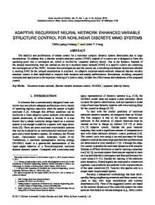
2.1 - ELMAN NETWORK ARCHITECTURE AND DYNAMICS Elman (1990) has proposed a partially recurrent network, where the feedforward connections are modifiable and the recurrent connections are fixed. Additionally to the input and the output units, the Elman network has a hidden unit, x h (k ) ∈ ℜ n and a context unit, x c ( k ) ∈ ℜ n . W x ∈ ℜ nxn , W u ∈ ℜ nxp and W y ∈ ℜ qxn are the interconnection matrices, respectively, for the context-hidden layer, input-hidden layer and hidden-output layer. Theoretically, an Elman network with n hidden units is able to represent a n th order dynamic system. However, due to practical difficulties with the identification of higher order systems, some modifications have been proposed. In Pham and Xing (1995) a selfconnection α ∈ ℜ + in the context unit is introduced, Figure 1, improving its memorisation ability.
u(k)
xh(k+1)
Wu
ϕ
Wy
Σ
yh(k+1)
x
W
D
Σ
xc(k+1) D
xc(k)
xh(k)
α
Figure 1: Block diagram of a modified Elman network. The dynamics of the modified Elman neural network is described by the difference equations (3)-(6). s( k + 1) = W x x c ( k + 1) + W u u ( k )
(3)
x h (k + 1) = ϕ { s (k + 1) }
(4)
x c ( k + 1) = x h ( k ) + α x c (k )
(5)
y h (k + 1) = W y x h (k + 1)
(6)
where s(k ) ∈ ℜ n is an intermediate variable and ϕ (⋅) is an hyperbolic tangent function. 2.2 - LEARNING METHODOLOGY The main difficulty related to the recursive training of recurrent networks arises from the fact that the output of the network and its partial derivatives with respect to the weights depend on the inputs since the beginning of the training process and on the initial state of the network. Therefore, a rigorous computation of the gradient, which implies taking into account all the past history is not practical. In this work, however, the gradient is approximated considering a finite number N of previous sampling periods. The training is defined on a sliding window mode, Henriques and Dourado (1998), where the identification criterion in the horizon [k − N ,K , k ] is defined by: E (k ) =
k
∑
e(i ) 2
(7)
i= k -N
where e( k ) ∈ ℜ q is the modelling error at time step k , given by: e( k ) = y ( k ) − y h ( k )
(8)
Several training algorithms have been proposed to adjust the weight values in recurrent networks. Examples of these methods are the dynamic backpropagation from Narendra and Parthasarathy (1991), the real time recurrent algorithm from Williams and Ziepser (1995) and the backpropagation through time from Werbos (1990), among others. This latest method is considered in the present work. For updating W x , W u and W y a gradient type algorithm is used as follows: ∂ E (k ) ∆W i (k+1) = ρ m ∆W i (k ) − µ m (1 − ρ m ) , i = u,x, y (9) ∂ W i (k ) where µ m ∈ ℜ + is the learning rate and ρ m ∈ ℜ + is a momentum term. The recurrent network is expanded into a multilayer feedforward network, being a new layer added at each time step. The computation of the derivatives in (9) is then performed as in the standard feedforward backpropagation network case, Rumelhart and Williams (1986), according to (10), (11) and (12). k ∂ E (k ) (10) δ h (i ) x c (i ) T = ∑ x ∂W i=k -N ∂ E (k ) ∂W
(11)
i= k-N
∂ E (k ) ∂W
k
∑ δ h (i) u(i − 1) T
=
u
y
k
=
∑
(12)
δ y (i) x h (i) T
i=k-N
The values of δ h (i ) ∈ ℜ n and δ y (i) ∈ ℜ q are computed recursively for i ∈ [k − N , k − 1] by (13)-(17). (13)
ε y (i ) = δ y (i ) = e(i )
(14)
T
ε h (i) = W y δ y (i ) + I n δ c (i + 1) δ h (i ) = ε h (i ) ⊗ ϕ ′{ s(i ) }
(15) (16)
T
ε c ( i ) = α I n δ c (i + 1) + W x δ h (i)
δ c (i ) = ε c (i ) The process is initialised at time k according to:
(17)
ε y ( k ) = δ y ( k ) = e(k ) = y( k ) - y h (k )
(18)
δ h ( k ) = ε h (k ) ⊗ ϕ ′{ s( k ) }
(19) (20)
T
ε c ( k ) = W x δ h (k )
The symbol ⊗ denotes the multiplication element by element, I n is an identity matrix and ϕ ′ (⋅) is the derivative of the hyperbolic tangent function ϕ (⋅) . 2.3 – INITIALISATION Considering the non-linear neural network (3)-(6), a linear model can be derived by a Taylor series expansion of (21) and neglecting the context unit contribution, yielding (22). (21) x h (k + 1) = ϕ W x x h ( k ) ,α W x x c ( k ) ,W u u ( k ) (22) x h (k + 1) = W A x h ( k ) + W B u (k )
{
where WA = WB
}
∂ ϕ {⋅ }
= diag [ϕ ′{⋅} ]W x
∂ x (k ) ∂ ϕ {⋅ } = = diag [ϕ ′{⋅}]W u ∂ u (k ) h
(23) (24)
Having a linear state space model describing the process to be identified (25)-(26) it is possible to provide previous knowledge to the network in order to initialise its weights, given the relationship between equations (22) and (25) and equations (26) and (6). (25) x( k + 1) = A x( k ) + B u (k ) y ( k ) = C x( k )
(26)
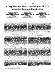
3. EXPERIMENTAL RESULTS 3.1 - THE HEATING SYSTEM In the laboratory process, depicted in Figure 2, air is forced to circulate by a fan blower through a duct and is heated at its inlet. This is a non-linear process with a pure time delay, which depends on the position of the temperature sensor element and the air flow rate, depending on the damper position Ω . The system input u (k ) , is the voltage on the heating device, which consists of a mesh of resistor wires, and the output, y (k ) , is the outlet air temperature.
Air Output
R
Ω
III
II
I
y(k)
u(k)
Output
Input Air Input
(a)
(b)
Figure 2: The Laboratory Process. (a) picture; (b) schematic diagram.
3.2 - EXPERIMENTS In order to assess the performance of the proposed on-line identification strategy a set of experiments was carried out. The experiments have been conducted using a common PC and the algorithms have been implemented in C code. For sampling time was chosen 0.25 second. In the experiments input variations and plant dynamics change have been considered. Additionally, the capability of prediction when the process identification is turned-off was also investigated. In all experiments the air damper was positioned at Ω = 10º and the sensor located at position III. Regarding the neural network, the number of hidden units (equal to the number of context units) is equal to three, n = 3 . For the truncated backpropagation learning algorithm the following parameters were chosen as: µ m = 0.02 , ρ m = 0.3 , α = 0.4 and N = 6. In Figure 3 are depicted the on-line identification with previous knowledge initialisation (a) and randomly initialisation (b). As can be seen, despite both initialisations are performing quite well, the one being carried out with previous knowledge exhibits a faster initial learning, as was expected.
35
25
60
yh(k)
20 y(k)
u(k) 40
15 0
5
10 15 Time [s]
(a)
20
30
80
30 25
60
y(k)
20
Input [%]
30
Temperature [ºC]
80 Input [%]
Temperature [ºC]
35
yh(k) u(k)
15 0
5
10 15 Time [s]
20
40 30
(b)
Figure 3: Identification (a) initial knowledge; (b) randomly initialisation. For different inputs, such as, square and sinusoidal waves, the proposed approach give results quite satisfactory as illustrated in Figure 4, even when varying the relevant characteristics of the waves (amplitude and frequency).
yh(k)
35
y(k)
20 y(k)
60
15 yh(k) 10
40
u(k)
5 0
20
Temperature [ºC]
25
Input [%]
80
40 60 Time [s]
30 60
25
Input [%]
30 Temperature [ºC]
80
35
20 15
40
u(k)
80
0
10
20
30
40
50
Time [s]
(a)
(b)
Figure 4: Identification (a) input square wave; (b) sinusoidal wave. In Figure 5 is illustrated the utilisation of neural modelling for prediction. In (a) an on-line identification with a sliding window N = 6 was carried out up to the instant 25 second, being the output prediction performed from instant 25 to 50 second, freezing the network weights. In (b) an off-line identification was performed at instant 37.5 second with data collected over one wave period, N = 100 (25 second), and the output predicted from this time on with this static neural model. As expected, the neural model is intimately dependent on the data set used for learning and thus can only be applied accurately for prediction in the same conditions of the data set training.
35
25
60
y(k)
20 yh(k)
0
10
20
30
30 60
yh(k)
25
y(k)
20
40
u(k)
15
u(k)
15
80 Input [%]
30
Temperature [ºC]
80
Input [%]
Temperature [ºC]
35
40 40
0
50
10
20
Time [s]
(a)
30 Time [s]
40
50
60
(b)
Figure 5: Identification and prediction (a) window size equal to 6; (b) window size equal to 100.
y(k)
25 20
60
yh(k) u(k)
Temperature [ºC]
30
35
80
30 25
60
y(k)
20 15
yh(k)
u(k)
40
40
15 0
20
40
60 80 Time [s]
(a)
100
120
0
10
20
30 40 Time [s]
(b)
Figure 6 : Identification (a) additional first order system; (b) additional time delay.
50
60
Input [%]
80
Input [%]
Temperature [ºC]
35
Finally, in Figure 6 is illustrated the plant dynamics modification with the inclusion of an additional first order system (constant time equal to 3 second) at instant 70 second, figure (a), and an additional one second delay, figure (b). As can be observed, the on-line neural learning performs very satisfactory in both cases, which reveals clearly the adaptive features of this methodology. Despite the identification behaviour in figure (b) is satisfactory, there exist at the beginning of each input transition an anticipation of the neural output. This is justified by the fact that the number of hidden unit is not enough for capturing the dynamics accurately. Experiments carried out using a higher number of hidden units reveal a superior performance and is not observed the reported behaviour.
4. CONCLUSIONS In this paper the application of a modified recurrent Elman network as general tool for modelling together with a truncated backpropagation through time algorithm for training have been presented. Given the simplicity of this network topology along with the fast training provided by the proposed learning algorithm, this approach is proved from the experiments on the laboratory plant, to be a feasible alternative for real-time identification. In this context, given the adaptive features revealed by the Elman networks as well their ability for modelling any kind of nonlinearities in the form of non-linear state space representation, they are bringing a valuable added-value to the control field and particularly to those strategies using an explicit model of the plant to be controlled. ACKNOWLEDGEMENTS This work was partially supported by the Portuguese Ministry of Science and Technology (MCT), under the program PRAXIS XXI.
REFERENCES Draye, J., Pavisic, D., Libert, G, 1996, “Dynamic recurrent neural networks: a dynamical analysis”, IEEE Trans. on Systems Man and Cybernetics, Part B, vol 26, nº 5, pp. 692-706. Elman, J., 1990, “Finding Structure in time“, Cognitive Science, 14, pp 1789-211. Filho, B., Cabral, E. Soares, A., 1998, “A new approach to artificial neural networks”, IEEE Trans. on Neural Networks, vol 9, nº 6, pp. 1167-1179. Henriques J.; Dourado, A., 1998, “A Multivariable adaptive control using a recurrent neural network” Proceedings of Eann98 – Engineering Applications of Neural Networks, Gibraltar, 9-12 June, pp 118-121. Hornik, K.; Stinchombe, M.; White, H., 1989, “Multilayer feedforward networks are universal approximators”, Neural Networks, 2, pp 359-366. Jin, L.; Nikiforuk, P.; Gupta, M., 1995, “Approximation of discrete time state space trajectories using dynamic recurrent networks”, IEEE Trans. Automatic Control, 40, nº 7, pp 1266-1270. Kosmatopoulos, E., Polycarpou, M., Iannou, A., 1995, “High-order neural network structures for identification of dynamical systems”, IEEE Trans. on Neural Networks, vol 6, nº 2, pp. 422-431. Linkens, D. Nyongesa, Y., 1996, “Learning systems in intelligent control: an appraisal of fuzzy, neural and genetic algorithm control applications”, IEE Proc. Control Theory App., 134 (4), pp 367-385. Narendra, K.; Parthasarathy, K., 1991, “Gradient methods for the optimisation of dynamical systems containing neural networks”, IEEE Trans. on Neural Networks, 2, nº 2, pp 252-262. Parlos, A., Chong, K., Atiya, A., 1994, “Application of the recurrent multilayer perceptron In modelling complex process dynamics”, IEEE Trans. on Neural Networks, vol 5, nº 2, pp. 255-266. Pham D.; Xing, L., 1995, “Dynamic System Identification Using Elman and Jordan Networks”, Neural Networks for Chemical Engineers, Editor A. Bulsari, Chap. 23, pp 572-591. Rumelhart, D.; Hinton, G.; Williams, R., 1986, “Learning internal representations by error propagation”, Explorations in the microstructure of cognition. Vol 1: Foundations, Cambridge, MIT Press/Bradford books. Werbos, P., 1990, “Backpropagation trough time, what it does and how do it“, Proc. IEEE, 78, pp 1550-1560. Williams, R.; Zipser, D., 1995, “Gradient-based learning algorithms for recurrent networks and their computational complexity”, Backpropagation, Edit by Yves Chauvin and D. Rumelhart, Chap.13, pp 433-486.