International Journal of Neural Systems World Scientific Publishing Company
APPLICATION OF NON-LINEAR AND WAVELET BASED FEATURES FOR THE AUTOMATED IDENTIFICATION OF EPILEPTIC EEG SIGNALS U RAJENDRA ACHARYA* Department of Electronics and Computer Engineering, Ngee Ann Polytechnic, Singapore 599489 S VINITHA SREE Global Biomedical Technologies, CA, USA ANG PENG CHUAN ALVIN Department of Electronics and Computer Engineering, Ngee Ann Polytechnic, Singapore 599489 RATNA YANTI Department of Electronics and Computer Engineering, Ngee Ann Polytechnic, Singapore 599489 JASJIT S. SURI Fellow AIMBE, CTO, Global Biomedical Technologies, CA, USA and Biomedical Engineering Department, Idaho State University (affl.), ID, USA (
[email protected]) *
Corresponding author: U R Acharya: Email:
[email protected]
Epilepsy, a neurological disorder, is characterized by the recurrence of seizures. Electroencephalogram (EEG) signals, which are used to detect the presence of seizures, are non-linear and dynamic in nature. Visual inspection of the EEG signals for detection of normal, interictal, and ictal activities is a strenuous and time-consuming task due to the huge volumes of EEG segments that have to be studied. Therefore, non-linear methods are being widely used to study EEG signals for the automatic monitoring of epileptic activities. The aim of our work is to develop a Computer Aided Diagnostic (CAD) technique with minimal pre-processing steps that can classify all the three classes of EEG segments, namely normal, interictal, and ictal, using a small number of highly discriminating nonlinear features in simple classifiers. To evaluate the technique, segments of normal, interictal, and ictal EEG segments (100 segments in each class) were used. Non-linear features based on the Higher Order Spectra (HOS), two entropies, namely the Approximation Entropy (ApEn) and the Sample Entropy (SampEn), and Fractal Dimension and Hurst Exponent were extracted from the segments. Significant features were selected using the ANOVA test. After evaluating the performance of six classifiers (Decision Tree, Fuzzy Sugeno Classifier, Gaussian Mixture Model, K-Nearest Neighbor, Support Vector Machine, and Radial Basis Probabilistic Neural Network) using a combination of the selected features, we found that using a set of all the selected six features in the Fuzzy classifier resulted in 99.7% classification accuracy. We have demonstrated that our technique is capable of achieving high accuracy using a small number of features that accurately capture the subtle differences in the three different types of EEG (normal, interictal, and ictal) segments. The technique can be easily written as a software application and used by medical professionals without any extensive training and cost. Such software can evolve into an automatic seizure monitoring application in the near future and can aid the doctors in providing better and timely care for the patients suffering from epilepsy. Keywords: epilepsy, Higher Order Spectra, non-linear analysis, entropies, ictal, interictal, electroencephalograms.
improve the quality of life of epileptic patients. The Electroencephalogram (EEG) signals are widely used to investigate brain disorders and to study brain electrical activity.31,47,55,56 The clinicians study the EEG segments for three types of electroencephalographic changes: ictal, which is usually characterized by continuous rhythmical activity that has a sudden onset when the patient is exhibiting a seizure; interictal, which is characterized by small spikes and subclinical seizures that generally occur during the time between seizures in epileptic patients; and normal EEG segments. Epilepsy monitors are commonly used to record long periods of EEG data for presurgical evaluation of epilepsy patients based on the occurrence of normal, interictal, and ictal activities. Detection of these activities by visual
1. Introduction Epilepsy is a common neurological disorder that causes the patient to have repeated seizures. Globally, between 4 and 10 per 1000 people are estimated to suffer from active epilepsy wherein the patients have continuing seizures and need treatment. In developed countries, between 40 and 70 per 100 000 people are diagnosed with epilepsy every year. However, in the case of developing countries, this figure is often close to twice as high due to the higher risk of experiencing conditions that can lead to permanent brain damage.63 Early and effective detection of epileptic activity will aid the clinicians in monitoring seizures and in administering appropriate seizure management protocols in order to 1
2
U Rajendra Acharya, Vinitha Sree S, Ang Peng Chuan Alvin, Jasjit S Suri
inspection of the EEG signals is a strenuous and timeconsuming task due to the huge volumes of EEG segments that have to be studied. Moreover, clinicians doing visual inspection require expert training and good experience in order to make credible predictions and avoid inter-observer variability. These issues can be addressed by developing Computer Aided Diagnostic (CAD) techniques that study the EEG segments and output the type of activity. Such automated techniques generally offer a faster, easier, more effective and affordable way to study epileptic activity. Many automated CAD techniques extract linear time-domain and frequency-domain based features from the EEG signals and use these features in classification models in order to determine the optimal feature subset and classifier combination that present the highest accuracy. However, since EEG signals are by nature non-linear,6-7,9,12,14-17,54,55 most of the recent studies1, 21,36,41,60 extracted non-linear features and used them in classifiers. The use of non-linear features based on Higher Order Spectra (HOS) of the EEG signals has been shown to provide good classification accuracy.21-23 Moreover, several studies37,48 have also evaluated the capabilities of entropies in detecting seizures. There are a few studies that extract features from the wavelet transform applied signals. These studies either focused on classifying only the normal and ictal classes48,53,59 or they used time frames or sub-bands of data.8,27-30 Details on the techniques employed in such CAD based epilepsy detection studies are provided in the discussion section of this paper. The results of these studies indicate that there is still room for improvement of classification accuracy. The aim of our work is to develop a technique with minimal pre-processing steps that can classify all the three classes of EEG segments, namely normal, interictal, and ictal, using a small number of highly discriminating non-linear features in simple classifiers. Such an automated technique can detect epilepsy because of its ability to classify normal and interictal activities, and can detect seizures in epilepsy monitoring units because of its capability to classify interictal and ictal segments. Thus, the objective of the work is to present to the clinicians an automated, simple, objective, fast, and cost-effective efficient secondary diagnostic tool that can aid in real-time monitoring of EEGs in order to provide additional confidence to their initial diagnosis of the class of the EEG segment. After sufficient clinical trials, such a tool
can evolve into a primary diagnostic tool for detection of epileptic EEG signals. The proposed technique, called (IntelligentWatch), is illustrated by a block diagram in Fig. 1. The offline system indicates the steps used for developing the classifiers. In this case, part of the original dataset, called the training dataset, is used for feature extraction. Features include entropies, HOS based features, Hurst exponent (H), and Fractal Dimension (FD). Highly discriminating features are selected using the Analysis of Variance (ANOVA) test and these feature vectors along with the ground truth that dictates the class of the sample are used to train classifiers. The classifiers learn the training parameters that best predict the class of the input sample. In the online real-time system that would be the end-product used in hospitals, no training of the classifiers is required. The significant features found in the training phase are extracted from the test sample, and the training parameters are applied on this feature vector to classify it into one of the three classes. The performances of the classifiers are reported as their accuracy, sensitivity, specificity, and Positive Predictive Value (PPV) registered for the test dataset. Normal, Interictal, and Ictal EEG segments (Training dataset) Feature Extraction: Entropies, HOS, H, FD Significant Feature Selection using ANOVA
Ground Truth
Offline Classification
Training Parameters
Normal, Interictal, and Ictal EEG segments (Test dataset)
Determination of significant features (similar to offline)
Online Classification
Normal
Ictal
Interictal
Offline system
Online system
Fig. 1 Block diagram of the proposed system (IntelligentWatch) for EEG classification; the blocks outside
2
Nonlinear features in epilepsy detection
The key novelty of this paper lies in the determination of highly discriminative combination of non-linear features that improve the classification accuracy to 99.7%. Such a high accuracy has not been reported by any studies in the literature. This paper is organized as follows: Section 2 presents the description of the data used in this work and provides brief description of the features and the feature selection technique. The classifiers and classification methodology are presented in Section 3. The feature selection results and the classification results are presented in Section 4. Section 5 presents a discussion on related studies and compares our results with other published work. The paper is concluded in Section 6.
pass filter. Typical normal, interictal, and epileptic (ictal) EEG signals are illustrated in Fig. 2. In this work, we selected 6 seconds data from each segment to develop an accurate classification framework for shorter segments. 1000
500
---> EEG (mcro volts)
the dotted shaded rectangular box represent the flow of offline training system, and the blocks within the dotted box represent the online real-time system.
3
0
-500
-1000
-1500
-2000
0
100
200
300
400
500 600 ---> Sample
700
800
900
1000
(a) 1000
2.1. EEG Data The EEG dataset used in this work was taken from the artifact free EEG time series data (Sets A, D, and E) available at the University of Bonn [see Andrzejak et al. 19 for more details]. EEG segments, each of length 23.6 seconds, were taken from five healthy subjects and five epileptic patients. For each of the three categories: normal (EEG segments taken from healthy subjects), interictal, and ictal/epileptic, 100 segments of the data were selected. Each EEG segment was considered as a separate EEG signal resulting in a total of 300 EEGs. The standard surface electrode placement scheme (the international 10-20 system) was used to obtain the normal segments from the five healthy cases (Set A recorded when patients were in the awake state with eyes open). Both the interictal and ictal segments were obtained from the five epilepsy patients undergoing presurgical evaluations. The interictal segments were recorded during seizure free intervals from the depth electrodes that were implanted into the hippocampal formations (Set D). The ictal segments were recorded from all sites exhibiting ictal activity using depth electrodes and also from strip electrodes that were implanted into the lateral and basal regions of the neocortex (Set E).19 All the segments were recorded using a 128-channel amplifier system, digitized with a sampling rate of 173.61 Hz and 12-bit A/D resolution, and filtered using a 0.53~40Hz (12 dB/octave) band
0
-500
-1000
-1500
-2000
0
100
200
300
400
500 600 ---> Sample
700
800
900
1000
700
800
900
1000
(b) 1000
500
---> EEG (micro volts)
2. Data and Methods
---> EEG (micro volts)
500
0
-500
-1000
-1500
-2000
0
100
200
300
400
500 600 ---> Sample
(c) 19
Fig.2. EEG signals (a) normal (b) ictal and (c) interictal
2.2. Feature Extraction Entropies Approximate Entropy (ApEn) Approximate Entropy is a measure of data regularity as it is defined as the logarithmic likelihood that the trends of the data patterns that are close to each other will remain close in the next comparison with next pattern. Highly regular data result in producing smaller ApEn values and vice versa. ApEn, proposed by Pincus et al.48,49 detects changes in the underlying episodic
4
U Rajendra Acharya, Vinitha Sree S, Ang Peng Chuan Alvin, Jasjit S Suri
Higher Order Spectra (HOS)-based features Higher Order Spectra based features quantify the nonlinear behaviour of a process.44,45 HOS features comprise of higher order moments (order greater than two) and nonlinear combinations of these higher order moments, called the higher order cumulants. The bispectrum, which is the spectrum of the third order cumulants, is one of the most commonly used HOS features. It is a complex valued function of two frequencies given by
behaviour that is not reflected in the amplitude or peaks of the signal. In order to calculate ApEn, consider a time series x(n), n= 1,2…,N. A series of patterns of length e (called the embedding dimension which is the smallest integer for which the patterns do not intersect with each other) is derived from x(n). ApEn is given by ApEn e, r , N
N e 1 1 1 N e log C ie r log C ie 1 r N e 1 i 1 N e i 1
(1) where the index r is a fixed parameter which sets the e tolerance of the comparison and Ci r is the correlation integral given by
Cie r
N e 1 1 r xi x j N e 1 j 1
where
B( f1 , f 2 ) E[ X ( f1 ) X ( f 2 ) X ( f1 f 2 )]
where X(f) is the Fourier transform of the signal and X* indicates the complex conjugate. As per the equation, the bispectrum is the product of the three Fourier coefficients. The function exhibits symmetry, and is computed in the non-redundant/ principal domain region Ω as shown in Fig. 3.
(2)
is
the Heaviside step function, and (a) 1a 0 . We chose r as 0.2 times the standard deviation of the time series, and e as 1.62 Since ApEn is very insensitive to low level noise it is very suitable for EEG signal analysis.
(a) 0a 0
Sample Entropy (SampEn) Sample Entropy, proposed by Richman et al.,52 is the negative natural logarithm of an estimate of the conditional probability that patterns of length e that match point-wise within a tolerance r also match at the next point.50 Even though SampEn is also a measure of data regularity like ApEn, SampEn is mostly independent of record length and displays relative consistencies under circumstances where ApEn does not.52 To calculate the sample entropy, runs of points matching within the tolerance r are carried out until there is no match, while the count of template matches are stored in counters A(k) and B(k) for all lengths k up to e. SampEn is given by the formula
A(k ) SampEnk , r , N ln B(k 1)
(4)
Fig. 3. Principal domain region (Ω) used for the computation of the bispectrum for real signals.
The Bispectral Phase Entropy (BPE),21-23 obtained from the bispectrum, is defined as
BPE n p(ψn )logp(ψn )
(5)
where
p( n )
1 l ( ( B( f1 , f 2 )) n ) L
n { | 2n / N 2 (n 1) / N },
(3)
n 0,1,..., N 1
where k = 0, 1,..., e-1 and B(0) N , the length of the input series. The k value was empirically chosen to be 5 in this work.57
(6) (7)
where L is the number of points within the region Ω,
is the phase angle of the bispectrum, and l(.) is an indicator function which gives a value of 1 when the phase angle is within the range depicted by n in equation (7). We also calculated two phase entropies which are similar to the bispectral phase entropy. They
4
Nonlinear features in epilepsy detection
are calculated as follows.21-22 Phase Entropy 1:
PhaseEnt1 pk logp k (8)
5
indicates the discrete time interval between points. The length for each of the k time series or curves was computed as:
k
where
pk
B( f1 , f 2 ) B( f1 , f 2 )
Phase Entropy 2:
{
PhaseEnt2 qi logqi
(9)
i
where
qi
B( f1 , f 2 )
2
B( f1 , f 2 )
2
In the above equations, the magnitude and the square of the magnitude are the L1 and L2 norms of the bispectrum and they were normalized by the sum of the norm over Ω such that each norm is now similar to a Probability Distribution Function (PDF) with values estimated from the Ω region. Due to the different nolinear dynamics existing in the three EEG classes, the normal, interictal, and ictal EEG are expected to have different PDF profiles of the bispectrum. We also calculated the Weighted Centre Of Bispectrum (Wcob),65 as follows,
f1m
iB(i, j) B(i, j)
f2m
∑
where i, j are the frequency bin index in the nonredundant region, f1m is Wcobx, and f2m is Wcoby. Higuchi Fractal Dimension The concept of fractal dimension (FD) originates from fractal geometry.42 FD is a powerful tool for transient detection and it can be used to measure the dimensional complexity of biological signals. It can give an indication of how completely the fractal appears to fill space. In this work, the algorithm proposed by Higuchi was used for finding FD of EEG signals.34 The EEG segment was assumed as a time sequence . Time series may be constructed as: (11) where m = 1, 2, …., k and int [ ] is an integer function. Here m indicates the initial time value and k
}
(12)
(13) Hurst Exponent (H) Hurst Exponent (H) is a measure of self-similarity, predictability and the degree of long-range dependence in a time-series. It is also a measure of the smoothness of a fractal time-series based on asymptotic behavior of the rescaled range of the process.26 According to the Hurst’s generalized equation of time series,35 H is defined as ( ⁄ )
(10)
| ⁄
where n is the total length of data sequence x. Mean value of the curve length was calculated for each by averaging for all m. Thus, an array of mean values was obtained. A plot of versus was made and FD was estimated from the slope of least squares linear best fit from the plot. Thus, FD can be defined as
jB(i, j ) B(i, j )
⁄ |
(14)
where T is the duration of the sample of data and is the corresponding value of rescaled range. R is the difference between the maximum and minimum deviation from the mean while represents the standard deviation.24 In other words, Hurst exponent is given by, ( ⁄ )
(15)
Here, is a constant and H is the Hurst exponent. Hurst exponent is estimated by plotting versus T in log-log axes. The slope of the regression line approximates the Hurst exponent. 2.3. Feature Extraction The extracted features are subjected to the one-way Analysis of Variance (ANOVA) test. In this technique, the variation of a feature between classes and the variation within a class are calculated. If the betweenclass variance is higher than the within-class variance,
6
U Rajendra Acharya, Vinitha Sree S, Ang Peng Chuan Alvin, Jasjit S Suri
algorithm33 is used to determine the parameters of the each Gaussian component and the weights of the mixtures based on the training data. The trained GMMs are used to classify the test data. In this work, we used a GMM containing five cluster centers.
the feature is considered to be statistically significant (low value of p). 3. Classification 3.1. Classifiers used
3.1.4. K-Nearest Neighbor (KNN)
In this work, we evaluated six classifiers namely Decision Tree (DT), Fuzzy Sugeno Classifier, Gaussian Mixture Model (GMM), K-Nearest Neighbor (KNN), Support Vector Machine (SVM), and Radial Basis Probabilistic Neural Network (RBPNN). They are briefly described in this section.
KNN is a supervised learning algorithm39 that uses the class labels of the neighbours of the new test data to predict the class of the test data. In the case of new test sample, K number of training points closest to the test sample are evaluated and the class that is most common amongst these K nearest neighbours is assigned as the class to the new test data. In this work, we varied the K nearest neighbors K=2 to 6. We obtained maximum accuracy for K= 2. The distance was computed using Euclidean distance.
3.1.1. Decision Tree (DT) A DT classifier40 is a decision support classifier that uses trees built using the input training dataset features. A series of rules are extracted from the tree and these rules are used to recognize the class of the test data. The parent node and leaf node values should be tuned, and in this work, we found that the parent and leaf node values of 6 and 1 respectively resulted in the highest accuracy.
3.1.5. Support Vector Machine (SVM) Support Vector Machine (SVM) is a supervised classifier whose main objective is to find a separating hyperplane that separates the training samples belonging to the three classes which are viewed in an ndimensional space (n is the number of features used as inputs) with a maximum margin between the hyperplane and the samples closest to the hyperplane (called the support vectors).25 If the data are not linearly separable, kernel functions can be used to map the original feature space to a higher dimensional feature space where the features become linearly separable. 43 In this work, we used the radial basis function kernel that has two training parameters: cost (C) which controls over-fitting of the model, and sigma (σ) which controls the degree of nonlinearity of the model. Using a grid search approach, we found that the accuracy was highest when C was 35, and sigma was set to 1.
3.1.2. Fuzzy Sugeno Classifier Fuzzy inference is a technique wherein the values in the input vector are interpreted based on a set of rules, and based on the interpretation, the input values are mapped to the output vector. In this work, during training, the subtractive clustering technique was used to generate a Fuzzy Inference System (FIS).61 This FIS structure contains the inputs, outputs, and a set of fuzzy rules that cover the feature space. These rules are then used to perform fuzzy inference calculations of the test data. In the FIS, the clusters were fixed using radii. It is a vector that specifies a cluster center's range of influence in each of the data dimensions, assuming the data falls within a unit hyperbox. Small radii values generally result in finding a few large clusters. The best values for radii are usually between 0.1 and 0.5. In our work, we have selected the radii of 0.4, the input membership function as 'Gaussian' and the output membership function as 'linear'.
3.1.6. Radial Basis Probabilistic Neural Network (RBPNN) RBPNN is a two-layer radial basis network18,38,64 used for classification.33 The first layer has radial basis activation functions which calculate the distance from the input test sample to the training input vectors and yields a distance vector. The next layer is the competitive layer which adds these distance vectors for each input classes and produces a vector of probabilities as its output.10, 13 The ‘compete’ transfer function at the
3.1.3. Gaussian Mixture Model (GMM) In the GMM classifier, the PDF of each class is assumed to consist of a mixture of multidimensional Gaussian distributions. The expectation-maximization
6
Nonlinear features in epilepsy detection
output of the second layer selects the maximum of these probabilities, and assigns a 1 for that selected class and a 0 for the other classes. All biases in the radial basis layer were set to √ , where s=spread constant of the RBPNN. In this work, we obtained maximum accuracy when s=0.5. 3.2. Classification methodology We have used a total of 300 EEG time series data segments (100 segments from each class). Seven significant features (as indicated in Table 1 in the Results section) were selected from these data to form the classification dataset. This classification dataset is used to build the classifiers. In order to develop robust classifiers that are adequately generalized to perform well when new samples are input, we chose the ten-fold cross validation data resampling technique for training and testing the classifiers. In this technique, the data is split into ten parts such that each part contains approximately the same proportion of class samples as the classification dataset. Nine parts of the data are used for training the classifier, and the remaining one part for testing. This procedure is repeated nine more times using a different part for testing in each case. Sensitivity, specificity, accuracy, and PPV are then calculated based on the results obtained for the test data in each folds. The average values of these performance measures over the ten folds are taken as the actual estimates of the classifier performance.
feature set and the classifier combination that presents the highest classification accuracy. Table 2 shows the results of accuracy, sensitivity, specificity, and PPV recorded by the six classifiers using all the six features. Our results show that the Fuzzy classifier performs better than the other classifiers by registering 99.7% for accuracy and 100% for sensitivity, specificity, and PPV. The results of this classifier for various other combinations of features are listed in Table 3. It is evident that on using all the six significant features, the maximum accuracy of 99.7% was registered indicating that all the features have a significant part in classifying the segments accurately. Table 1 Range (Mean ± Standard Deviation) of features for normal, interictal, and ictal EEG classes. Features
ApEn SampEn
PhaseEnt2 Wcoby FD H
4. Results We calculated ApEn, SampEn, and in the case of HOS features, we found the BPE, PhaseEnt1, PhaseEnt2, Wcobx, Wcoby, and we also determined Hurst Exponent (H) and Higuchi Fractal Dimension (FD). ANOVA was used to determine the significant features. Table 1 shows the range of selected six features for normal, interictal, and ictal classes. ApEn and SampEn were both found to be significant as indicated by the low pvalues. Among the HOS features, PhaseEnt2 and Wcoby were found to be significant. Both H and FD were also significant features. The entropy features (SampEn and ApEn) have lower values for the abnormal (ictal and interictal) classes compared to the normal class. Such varied ranges for each feature indicate that various combinations of these features should be evaluated in each of the classifiers to determine the
7
Normal
Interictal Entropies 2.202 1.8178 ± ±3.546E-02 0.170 1.3180 ± 1.0301 ± 0.114 0.133 HOS
Ictal 1.8343 ± 0.209 0.91719 ± 0.122
0.45268 ±8. 433E-02 10.365 ± 10.7
0.28522 ± 8.369E-02 3.3568 ± 1.70
0.33037 ± 0.179 8.3844± 2.55
-1.4695 ± 9.093E-02 0.66828 ± 8.706E-02
-1.2919 ± 8.128E-02 0.79709± 5.445E-02
-1.3286 ± 0.124 0.52875 ± 0.122
p-value