Application of Resilient Back-Propagation Neural Networks for

Available online at http://ejournals.uofk.edu UofKEJ Vol. 1 Issue 2 pp. 9-21 (October 2011)

UNIVERSITY of KHARTOUM ENGINEERING JOURNAL (UofKEJ)

Application of Resilient Back-Propagation Neural Networks for Generating a Universal Pressure Drop Model in Pipelines Mohammed A. Ayoub, Birol M. Demiral University Teknologi Petronas, Petroleum Engineering Department Bandar Seri Iskandar 32610, Perak –Malaysia (E-mail: [email protected]) Abstract: This study aims at generating and validating a universal pressure drop model at pipelines under threephase flow conditions. There is a pressing need for estimating the pressure drop in pipeline systems using a simple procedure that would eliminate the tedious and yet the non accurate and cumbersome methods. In this study resilient back-propagation Artificial Neural Network technique will be utilized as a powerful modeling tool to establish the complex relationship between input parameters and the pressure drop in pipeline systems under wide range of angles of inclination. A total number of data points consists of 335 sets has been used for generating, validating, and testing the ANN model. A model performance has been evaluated against the best empirical correlations and mechanistic models (Xiao et al., Gomez et al., and Beggs and Brill). A series of statistical and graphical analysis were conducted to show the significance of the generated model. The new developed model outperforms all investigated models with correlation coefficient reaches 98.82%. Keywords: Artificial Neural Networks; resilient back-propagation; Multiphase flow; pressure drop; universal model. . A thorough literature survey has been done in the area of pressure drop estimation in multiphase system. Current empirical correlations and mechanistic models were reviewed and their drawbacks have been stated [1]. A critical and thorough literature survey of available technical and published papers has resulted in many models used for estimating pressure drop in pipelines. However, few of them are designed to estimate the pressure drop at all angles of inclination. Only the best models will be selected to compare their performances against the new developed model. Beggs and Brill Model [2] was derived from a huge number of database (584 data points) but in a small scale test facility where air and water were used as testing fluids using 1 inch and 1.5 inches diameter pipes. The model was made to serve for all angles of inclination ranging from -90 to 900. The factors used for correlating are gas flow rate, liquid flow rate, pipe diameter, inclination angle, liquid holdup, pressure gradient and horizontal flow regime (segregated, intermittent and distributed).

1. INTRODUCTION Two phase flow; namely liquid and gas, or what is alternatively called Multiphase flow, occurs in almost all oil production wells, in many gas production wells, in some types of injection wells, and in pipelines with different configurations. Multiphase flow mixture can be convoyed horizontally, vertically, or at any angle of inclination. However, defining the pressure profile as a general case for all these configurations has some limitations in relation to changing liquid hold-up and flow patterns, slippage criterion, and friction factor determination. Velocity profile of each phase is hard to be determined inside the pipe facility. The pressure drop (DP) mainly resides between well head and separator facility. This pressure drop needs to be estimated with a high degree of precision in order to execute certain design considerations. Such considerations include tube sizing, operating wellhead pressure in a flowing well, direct input for surface flow line and equipment design calculations. Determination of pressure drop is very essential because it provides the designer with the suitable and applicable pump type for a given set of operational parameters. In addition, it can be used as a guideline for the operational cost estimation in terms of pipeline sizing. Generally, the proper estimation of pressure drop in pipeline can help in the design of gas-liquid transportation systems.

A study conducted in Kuparuk field indicated that Begs & Brill predict pressure drop with 10% accuracy for all production pipelines, [3]. While a recent study showed that Beggs and Brill correlation always over predicts pressure gradients, [4]. Yuan and Zhou conducted a comparative study for many pressure prediction correlations and mechanistic models that are widely used by the industry utilizing experimental data with seven angles of inclination. However, 9

Mohammed A. Ayoub and Birol M. Demiral / UofKEJ Vol. 1 Issue 2 pp. 9-21 (October 2011) and Flangian and Eaton. Finally, for a pipeline with 2-inches in diameter the authors concluded that Xiao model was the best, followed by Eaton.

the authors claimed that their study can be used as a guideline for selecting two-phase flow pressure drop prediction correlation and mechanistic model in designing and analyzing downward two-phase flow pipelines.

The overall objective of this study is to minimize the uncertainty in the multi-phase pipeline design. This is achieved by developing a representative model for pressure drop determination in downstream facilities with the use of the most relevant input variables and a wide range of angles of inclination. Specific objective is: − To construct and test two models for predicting pressure drop in pipeline systems under multiphase flow conditions with real field data for a wide range of angles of inclination (from -520 to 2080) using Artificial Neural Networks techniques.

Xiao et al. Model [5] is a comprehensive mechanistic model designed for gas-liquid two phase flow in horizontal and near horizontal pipelines. Among its numerous benefits, the model can predict the pressure drop in pipeline with high degree of accuracy compared to other tested correlations and models. The model performance has been evaluated against the data bank collected from the A.G.A database and laboratory data published in literature. Begs and Brill correlation was found to perform the best over three tested models named Dukler et al., Dukler-Eaton, and Mukherjee and Brill [5]. The mechanistic model developed by Xiao et al. [5] has been used as a base for another model expanded by Manabe et al. [6]. An experimental program was set up to cover all the flow patterns. Three models were used for testing the mechanistic model performance. Beggs and Brill correlation ranked second after Dukler et al model. However, Mukherjee and Brill model proved to be the least accurate among the tested models.

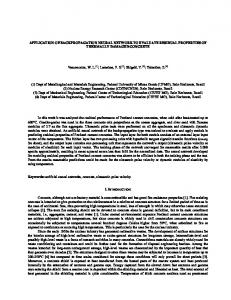
2. METHODOLOGY The methodology involves filling the gap does exist in the literature by assessing and evaluating the best multiphase flow (MPF) empirical correlations and mechanistic models. The assessment will be dealing with their performance in estimating pressure drop whilst using available statistical and graphical techniques. The performance of the proposed model will be compared to the best available correlations used in the industry. Fig. 1 illustrates the sequence of research events.

Gomez et al. [7] presented a comprehensive model for prediction of flow pattern, liquid holdup and pressure drop in wellbores and pipelines. The model is valid for inclination angles range from horizontal to upward vertical flow. The model has been validated using laboratory and field data. Furthermore, the model has been tested against field data, from the North Sea and Prudhoe Bay, Alaska. The model’s pressure drop performance also has been compared to other six models and showed significant results.

Data collection and partitioning, filtering and screening procedure, data randomization, pre-processing, and postprocessing were all done before running the models. A total number of 338 data sets have been utilized for the purpose of this study for modeling ends (range of collected data has been presented in Appendix B). Only three data sets have been removed as outliers according to the semi-studentised residual or (standard residual). * ei ei = (1) MSE

Petalas and Aziz, [8] developed a comprehensive mechanistic model using a large set of data from Stanford Multiphase Database. Their model was able to identify flow regimes based on certain assumptions. Additionally, it is applicable to a wide range of fluid properties and pipe geometries. The model also incorporated roughness effects as well as liquid entrainment, which were not considered by previous models. The authors finalized their effort by making the model able to calculate the pressure drop at any flow pattern and to calculate the liquid volume fraction efficiently. Hong and Zhou [9] presented a comprehensive review of the applicability of some empirical and mechanistic models using commercial software. Data from published work have been used for this purpose. Five empirical correlations and a single mechanistic model were chosen by the authors to compare their model’s performance; those are Beggs-Brill, DuklerEaton-Flanigan, Dukler-Flanigan, Dukler, Eaton, and EatonFlanigan correlations and Xiao et al mechanistic model. The authors concluded that Beggs-Brill correlation always overestimates the pressure gradient in all studied cases. However, for small pipe diameter with superficial-liquid velocities greater than 3 ft/sec the authors noticed that Dukler behaves the best, followed by Xiao and Eaton and Flangian. Moreover, at Superficial Liquid Velocities less than 3 ft/sec, they reported that Xiao behaves the best, followed by Eaton

*

where; ei is the semi-studentised residual (or standard residual); MSE is the mean square error of the data; e i is the residual (difference between actual and predicted values). Relevant input variables were selected based on the most commonly used empirical correlations and mechanistic models in the industry. Eight attributes are thought to have a strong impact on the pressure drop estimation, which are; oil rate, water rate, gas rate, diameter of the pipe, length of pipe, wellhead pressure, wellhead temperature, and angle of deviation. Oil viscosity and density were found ineffective due to low range of data used. However, the model accuracy and consistency have not been affected. The data have been partitioned into three sets; training, validation, and testing. By definition, the training set is used to develop and adjust the weights in a network. The validation set is used to ensure the generalization of the developed network during the training phase, and the test set is used to examine the final 10

Mohammed A. Ayoub and Birol M. Demiral / UofKEJ Vol. 1 Issue 2 pp. 9-21 (October 2011) has never been seen by the network during the training sessions. The developed model consists of one input layer (containing a specific number of input neurons or nodes), which represents the parameters involved in estimating pressure drop. One or two hidden layers contain a certain number of neurons and one output layer contains one node, which is pressure drop at the outlet. The model also contains an activation state for each unit, which is equivalent to the output of the unit. An activation function will be applied to find out the new level of activation based on the effective input and the current activation. Additional term is included, which is an external input bias for each hidden layer to offer a constant offset and to minimize the number of iterations during the training process. 2.1 Data Transformation Data transformation is used for ANN model where all data samples have been transformed or scaled to fall within a prespecified range. This step is crucial before generating a successful ANN model because it eliminates the harmful effect of varied input ranges. This step is needed to transform the data into a suitable form to the network inputs and targets. The approach used for scaling network inputs and targets was to normalize the training set through using mapminmax builtin function in Matlab within a pre-specified range [-1, 1]. The function can be mathematically expressed with the following equation: y=

( y max − y min )( x − xmin ) + y min ( xmax − xmin )

(2)

In order to transform the x value to y value, the above formula has to be implemented provided that the range of the data falls between ymin and ymax [10]. , 2.2 The Resilient Back-propagation Algorithm (RPROP)

Fig. 1. Detailed research methodology of the current study performance of the network. The primary concerns should be to ensure two things: (a) the training set contains enough data, and suitable data distributed evenly to cover the entire range of data, and (b) there is no unnecessary similarity between the data in different sets [11].

The algorithm acts on each weight separately. For each weight, if there was a sign change of the partial derivative of the total error function compared to the last iteration, the update value for that weight is multiplied by a factor η−, where 0 1. The update values are calculated for each weight in the above manner, and finally each weight is changed by its own update value, in the opposite direction of that weight's partial derivative. This is to minimize the total error function. η+ is empirically set to 1.2 and η− to 0.5.

With respect to ANN model, different partitioning ratios have been tested before finally selecting one for the specific model (2:1:1, 3:1:1, and 4:1:1). The ratio of 4:1:1 is known to yield better training and testing results (but depends on the number of data set used for training), [11]. The problem with this ratio is that it is not frequently used by researchers. Instead, a ratio of 2:1:1 between the three sets has been followed for this study. This ratio coincides with one half of the data reserved for training. One quarter of the data has been kept for validation while the remaining quarter has been allocated for testing the network performance. This categorization is corresponding to 168 data sets reserved for training the model while 83 data sets were utilized for validation purposes. The other 84 data set has been kept aside for testing the new model performance. Needless to mention that this testing set

To elaborate the above description mathematically we can start by introducing for each weight w ij its individual updatevalue ∆ ij (t) , which exclusively determines the magnitude of the weight-update. This update value can be expressed mathematically according to the learning rule for each case based on the observed behavior of the partial derivative during two successive weight-steps by the following formula: 11

Mohammed A. Ayoub and Birol M. Demiral / UofKEJ Vol. 1 Issue 2 pp. 9-21 (October 2011) ⎧ + ⎪η ⋅ ∆ij (t −1), ⎪ ⎪⎪ ∆ij (t) = ⎨η− ⋅ ∆ij (t −1), ⎪ ⎪∆ (t −1), ⎪ ij ⎩⎪

if

∂E ∂E (t) ⋅ (t −1) > 0 ∂wij ∂wij

if

∂E ∂E (t) ⋅ (t −1) < 0 ∂wij ∂wij

training patterns, [12]. It is noticed that resilient backpropagation is much faster than the standard steepest descent algorithm. Resilient back-propagation (RPROP) training algorithm was adopted to train the proposed ANN model as mentioned previously.

(3)

else

2.3 Network Selection

Different network topologies have been tried in an attempt to find the optimum network architecture. Among them, backpropagation network with feed-forward algorithm gained pronounced publicity in solving hard problems, especially in petroleum engineering. However, back-propagation network with feed-forward cycle reported to have several shortcomings. One of the main problems associated with this type of networks is its trapping in local minima instead of global one. In addition, slow convergence is witnessed when the network fails in several occasions to converge to the optimum solution. To avoid such shortcomings, resilient back-propagation network (special type of general backpropagation scheme) has been tried in this study in an attempt to generate a successful model for estimating pressure drop in pipeline with a wide range of angles of inclination. This algorithm is working under the scheme of local adaptive learning for supervised learning feed-forward neural networks. The reason for selecting such a network topology is its fast convergence compared to other networks. In addition, contrary to other gradient descent algorithms which count for the change of magnitude of weight derivative and its sign; resilient back-propagation only counts for the sign of the direction of weight.

where 0 < η− < 1 < η+ . A clarification of the adaptation rule based on the above formula can be stated. It is evident that whenever the partial derivative of the equivalent weight w ij varies its sign, which indicates that the last update was large in magnitude and the algorithm has skipped over a local minima, the update-value − ∆ ij (t) is decreased by the factor η . If the derivative holds its sign, the update-value will to some extent increase in order to speed up the convergence in shallow areas. When the update-value for each weight is settled in, the weight-update itself tracks a very simple rule. That is if the derivative is positive, the weight is decreased by its updatevalue, if the derivative is negative, the update-value is added:

⎧ ⎪− ∆ ij (t ), ⎪ ⎪⎪ ∆wij (t ) = ⎨∆ ij (t ), ⎪ ⎪0, ⎪ ⎪⎩

∂E (t ) > 0 ∂wij

if if

∂E (t ) < 0 ∂wij

(4)

else

wij (t + 1) = wij (t ) + ∆wij (t )

2.4 Network Training

(5)

However, there is one exception. If the partial derivative changes sign that is the previous step was too large and the minimum was missed, the previous weight-update is reverted:

∆wij (t ) = −∆wij (t − 1), if

∂E ∂E (t ) ⋅ (t − 1) < 0 ∂wij ∂wij

(6)

Due to that ‘backtracking’ weight-step, the derivative is assumed to change its sign once again in the following step. In order to avoid a double penalty of the update-value, there should be no adaptation of the update-value in the succeeding step. In practice this can be done by setting the

∆ ij

∂E (t − 1) = 0 ∂w ij

in

update-rule above.

The partial derivative of the total error is given by the following formula:

∂E 1 P ∂E p (t ) = (t ) ∂wij 2 p =1 ∂wij

∑

(7)

Hence, the partial derivatives of the errors must be accumulated for all training patterns. This indicates that the weights are updated only after the presentation of all of the 12

The network has been trained using resilient backpropagation training scheme. The training parameters have been modified several times until the optimum performance has been achieved. In this part a number of modified training parameters will be presented along with justification for each case. Maximum number of iterations has been set to 500 epochs since the resilient back-propagation is famous of its fast convergence. After small number of iterations, the network converges to the optimum solution. Maximum validation failures have been set to 6 cases only since great number of failed validation cases may affect the network stability and generality when new cases are presented to the network. Learning rate is used to enhance the training speed and efficiency. This factor has been varied between the values of 0.5 to 1.5 while the performance is monitored carefully. A value of 1.05 is found to achieve the fastest and most efficient training performance. However, the increase and decrease factors η+ and η− are set to fixed values: η− =0.5 and η + = 1.2 . These are reported in Matlab script as (net.trainParam.delt_dec =0.5 & net.trainParam.delt_inc =1.2). Initial weight change is kept at its default value (net.trainParam.delta0 =0.07) to avoid the escalating values of weights. The maximum weight-step determined by the size of the update-value is limited. The upper bound is set by the second parameter of RPROP, ∆ max . The default upper bound is set somewhat arbitrarily to ∆ max = 50.0 and it is reported in

Mohammed A. Ayoub and Birol M. Demiral / UofKEJ Vol. 1 Issue 2 pp. 9-21 (October 2011) Matlab script as (net.trainParam.deltamax= 50). Usually, the convergence is rather insensitive to this parameter as well. The minimum step size is always fixed to a value ∆ min = 1e −6 .

performance. Selection of an objective function is very important because it represents the design goals and decides what training algorithm can be taken. A few basic functions are commonly used. One of them, used in this study, is the sum of the squares of the errors.

2.5 Output Post-Processing (Denormalization)

This step is set for presenting results of ANN model. This step is the most important task after the model has been generated. This was needed to transform the outputs of the network to a comprehensible value by reverting the original value used. It is the stage that comes after the analysis of the data and is basically the reverse process of data preprocessing.

where, p refers to patterns in the training set, k refers to output nodes, and opk and ypk are the target and predicted network output for the kth output unit on the pth pattern, respectively.

2.6 Network Performance Comparison

3. RESULTS AND DISCUSSION

Pressure drop calculation for Beggs and Brill correlation, Gomez et al. model, Xiao et al. model has been conducted using an executable code that programmed using FORTRAN language. The code allows great flexibility in selecting PVT methods, type of pressure drop correlation (vertical, inclined, and horizontal), operating conditions, and flow-rate type data. Only test data has been chosen for comparing each selected model against the proposed ANN model. The network performance comparison has been conducted using the most critical statistical and analytical techniques. Trend analysis, group error analysis, and graphical and statistical analysis are among these techniques.

Neural network model for estimating pressure drop in pipelines has been already built and optimized after a series of model runs. The modeling process starts by optimizing the best architecture that achieves the best performance. For pressure drop estimation, only Beggs and Brill correlation [2], Xiao et al. [5], and Gomez et al. [7] models will be used to compare the generated model performance. Trend analysis for generated model will be conducted and assessed. Matlab software [19] will be utilized for generating codes of the program. The final performance has been thoroughly addressed through applying a series of statistical and graphical error analyses.

2.7 ANN Model Architecture

3.1 ANN Model Optimization

This model can be defined with number of layers, the number of processing units per layer, and the interconnection patterns between layers. Therefore, defining the optimal network that simulates the actual behavior within the data sets is not an easy task. To achieve this, certain performance criteria were followed. The design started with adding a few numbers of hidden units in the first hidden layer that acts as a feature detector. The basic approach used in constructing the successful network was trial and error. The generalization error of each inspected network design was visualized and monitored carefully through plotting the governing statistical parameters such as correlation coefficient, root mean squared errors, standard deviation of errors, and average absolute percent error of each inspected topology. Another statistical criterion, maximum validation error was utilized as a measure of accuracy of the training model. Besides, a trend analysis for each inspected model was conducted to see whether that model simulates the real behavior. Data randomization is necessary in constructing a successful model, with a frequent suggestion that input data should describe events exhaustively. This rule of thumb can be translated into the use of all input variables that are thought to have a problemoriented relevance. These eight selected input parameters were found to have pronounced effect in estimating pressure drop.

The optimum number of hidden units depends on many factors: the number of input and output units, the number of training cases, the amount of noise in the targets, the complexity of the error function, the network architecture, and the training algorithm. In most cases, there is no direct way to determine the optimal number of hidden units without training using different numbers of hidden units and estimating the generalization error of each.

Error =

1 NP

P

N

∑ ∑ ( y pk − o pk ) 2

(8)

p =1 k =1

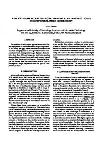
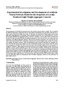
Figs 2 and 3 illustrate the effect of changing the number of neurons in the first hidden layer on the average absolute percent error and correlation coefficient, respectively. As observed from Fig. 2, one hidden layer with nine hidden neurons achieved the highest correlation coefficient and the lowest average absolute percent error. But, on the other hand, the model failed in producing the correct physical trend across the data range. Instead, additional hidden layer was added and the number of hidden nodes was increased gradually until the correct trend was achieved. The selection of this model was based on having the highest correlation coefficient for the training and validation sets. But still the performance of the model is not good enough and the inherent relationship between input variables and the output is not well extracted. The whole procedure was discarded when it was found that obtaining the right trend cannot be achieved easily through application of traditional backpropagation training algorithms such as gradient descent, and gradient descent with momentum. They are very slow in nature compared to other fast, practical, and high performance algorithms such as resilient back-propagation. The latter has been used in training the model.

2.8 Objective Function for ANN Model

To train the network and measure how well it performs, an objective function (or cost function) must be defined to provide an explicit numerical rating of the system 13

4.0

AAPE-Va lida tion

AAPE-Tra ining

AAPE-Testing

3.5

3.0

2.5

2.0 2 hidden

4 hidden

6 hidden

8 hidden

9 hidden

Fig. 2. Effect of changing Number of Neurons on average absolute percent error. 0.9994

Correlation Coefficient (fraction)

Each topology which failed to produce the correct physical trend has been discarded. Only three successful topologies have been recorded and prepared for comparison. The first model consists of seven hidden nodes in the first hidden layer while the second model consists of twelve hidden nodes in the first hidden layer. The performance of these two networks was not up to satisfaction. It is decided to increase the number of the hidden layers to reach two and slightly increasing the number of hidden nodes until we capture a topology that represents the inherent relationship between the input parameters and the target output. Only one structure was successful in producing the correct physical trend which was a network of nine nodes in the first hidden layer and four in the second hidden layer. Results of successful networks in terms of average absolute percent error and correlation coefficient are tabulated in Table 1(Appendix A). However, maximum error of each set is presented as a good governing statistical criterion for selecting the model of the lowest value, is tabulated in Table 2 (Appendix A). In addition, Table 3 (Appendix A) presents the root mean square errors and standard deviations of errors for the validation and testing sets which will aid in selecting the best model with the lowest value.

Average Absolute Percent Error (%)

Mohammed A. Ayoub and Birol M. Demiral / UofKEJ Vol. 1 Issue 2 pp. 9-21 (October 2011)

R-Testing

R-Validation

0.9993 0.9992 0.9991 0.999 0.9989 0.9988 0.9987

Fig. 4 shows the effect of changing number of neurons on average absolute percent error for training, testing and validation sets while using resilient back-propagation training algorithm. Fig. 5 shows the effect of changing the number of neurons on maximum error for each set using resilient backpropagation training algorithm. It is clear from this figure that the topology 8-9-4-1 presents the lowest maximum error for all data sets. Fig. 6 shows the effect of changing the number of neurons on correlation coefficient for each set using resilient back-propagation training algorithm. Again, the previously mentioned topology achieved the highest correlation coefficients for all data sets. Fig. 7 depicts the effect of changing the number of neurons on root mean square errors for testing and validation sets using resilient back-propagation training algorithm. In this time validation and testing sets were used as they are verifying the model performance while training set is neglected because output is seen by the network during training. Using these two sets, the same architecture (8-9-4-1) succeeded in producing the lowest root mean square errors compared to the other two topologies.

2 hidden

4 hidden

6 hidden

8 hidden

9 hidden

Average Absolute Percent Error, (%)

Fig. 3. Effect of changing Number of Neurons on correlation coefficient 26 24

AAPE-train

AAPE-valid

AAPE-test

22 20 18 16 14 12 10 8-9-4-1 Network

8-7-1 Network

8-12-1 Network

Fig. 4. Effect of changing Number of Neurons on average absolute percent error using resilient back-propagation training algorithm 440

Fig. 8 illustrates the effect of changing the number of neurons on standard deviation of errors for testing and validation sets using resilient back-propagation training algorithm. In this figure the architecture of 8-9-4-1 neurons was capable of attaining the lowest standard deviation of errors among all tested topologies. From the previously presented discussion and figures it is clear that the topology of 8-9-4-1 achieved the optimum performance among all topologies. However, all statistical features used to assess the performance of all investigated architectures demonstrated that two hidden layers with nine and four hidden nodes are quite sufficient to map the relationship between the input variables and the total output (pressure drop). This final selection of model topology

Maximum Error Per Set, (psia)

390

Val-Max-Error

Test-Max-Error

Train-Max-Error

340 290 240 190 140 90 40 8-9-4-1 Network

8-7-1 Network

8-12-1 Network

Fig. 5. Effect of Changing Number of Neurons on Maximum Error for each set using Resilient Back-Propagation Training Algorithm.

14

Mohammed A. Ayoub and Birol M. Demiral / UofKEJ Vol. 1 Issue 2 pp. 9-21 (October 2011)

Correlation Coefficient Per Set

3.2 Trend Analysis R-Testing

R-Validation

R-training

0.990

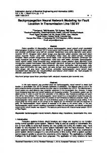
A trend analysis was carried out to check whether the developed model is physically correct. To test the developed model, the effects of gas rate, oil rate, water rate, tubing diameter, angle of deviation and pipe length on pressure drop were determined and plotted on Figs. 9 through 14. The effect of angle of inclination was investigated where each parameter was plotted against pressure for different angles of inclination. This can be demonstrated in Fig. 9, which shows the effect of changing gas rate on pressure drop values. As expected, the developed model produced a correct trend where the pressure drop increases as the gas rate increases. However, a justification is needed at low gas flow rate at vertical pipe. The Fig. must show that the pressure drop should be higher than for other less valued angles. The reason for such behavior is that if the line is not horizontal, an increase in gas velocity will sweep some of the liquid accumulation at the lower sections of the pipe, which might lead to an overall decrease in pressure drop, [13].

0.980 0.970 0.960 0.950 0.940 8-9-4-1 Network

8-7-1 Network

8-12-1 Network

Root Mean Square Error Per Set

Fig. 6. Effect of changing Number of Neurons on correlation coefficient for each set using Resilient Back-Propagation Training Algorithm. RMSE-Testing

RMSE-Validation

50.9 40.9

This finding is compatible with the physical phenomenon according to the general energy equation as stated in the following formula:

30.9 20.9

dP g fρυ 2 ρυdυ = + ρ sin θ + dL g c 2 g c D g c dL

10.9 0.9 8-9-4-1 Network

8-7-1 Network

8-12-1 Network

where; g ρ sin θ = pressure gradient due to elevation or potential gc energy change, fρυ 2 = pressure gradient due to frictional losses, 2g c D ρυdυ = pressure gradient due to acceleration or kinetic g c dL energy change,

Fig. 7. Effect of changing Number of Neurons on root mean square errors for testing and validation sets using Resilient Back-Propagation Training Algorithm 16 Sta nda rd Devia tion Per Set

STD-Testing

(9)

STD-Validation

15 14 13

P = pressure, lbf/ft2 L = pipe length, ft g = gravitational acceleration, ft/sec2 gc = 32.17, ft-lbm/lbf-sec2

12 11

ρ

= density lbm/ft3 θ = dip angle from horizontal direction, degrees

10 8-9-4-1 Network

8-7-1 Network

8-12-1 Network

f

= Darcy–Wiesbach (Moody) friction factor

υ = flow velocity, ft/sec

Fig. 8. Effect of changing Number of Neurons on standard deviation of errors for testing and validation sets using Resilient Back-Propagation Training Algorithm

D = pipe inner diameter, ft If the second and third term of the abovementioned equation is considered, the flow velocity is incorporated in the numerator of each term, which indicates that the pressure drop is directly proportional to the flow velocity and; Q (10) υ= A As indicated in equation 10 while the cross sectional area is fixed for a given pipe size the velocity term can be used

is further assessed through conducting a trend analysis. Input weight matrix (from input to the hidden layers), hidden layer weight matrices, and the layers bias vectors for the retained network, all are extracted from this program and presented in Appendix B. These weights and biases can be utilized in developing an executable code, which provides an easy way for users to implement in predicting pressure drop.

15

Mohammed A. Ayoub and Birol M. Demiral / UofKEJ Vol. 1 Issue 2 pp. 9-21 (October 2011) 140

190 ∆[email protected]⁰

∆[email protected]⁰

∆[email protected]⁰

∆P@90⁰

130

170

120

150

Pressure Drop (Psia)

Pressure Drop (Psia)

∆P@90⁰

110 100 90

∆[email protected]⁰

∆[email protected]⁰

∆P@‐20.0⁰

130 110 90 70

80

50

70

30 500 Gas Flowrate  (MSCF/D)

3,411

6,322

9,233

12,144 15,056 17,967 20,878 23,789 26,700

Length of the pipe (ft) 

Fig. 9. Effect of gas rate on pressure drop at four different angles of inclination.

Fig. 13. Effect of pipe length on pressure drop at four different angles of inclination. 210

∆P@90⁰

∆[email protected]⁰

∆[email protected]⁰

∆P@‐20.0⁰

∆P@ 6.065''

160 140

∆P@ 9.2''

∆P@ 10.02''

170

Pressure Drop (Psia)

Pressure Drop (Psia)

∆P@ 8.7''

190

120 100 80 60

150 130 110 90

40

70

20

50 Angle of Deviation (deg) 

Oil Flowrate (bbl/d) 

Fig. 10. Effect of oil rate on pressure drop at four different angles of inclination.

Fig. 14. Effect of angle of inclination on pressure drop at four different pipe piameters.

120 115

∆P@90⁰

∆[email protected]⁰

∆[email protected]⁰

∆P@‐20.0⁰

interchangeably with flow-rate. This expression is valid for oil flow-rate, gas flow-rate, and water flow-rate. The ANN model succeeded in producing the right trend for the three phases (gas, oil, and water) as illustrated in Fig. 9, Fig. 10, and Fig. 11, respectively.

Pressure Drop (Psia)

110 105 100 95 90 85

Another observation is reported where the pressure drop is found to be an increasing function with respect to angle value for all three phases, which is physically sound and follows the normal trend. The pressure drop has been plotted against each phase rate (oil flow-rate, water flow-rate, and gas flowrate) for different four configurations (horizontal, vertical, inclined hilly terrain, and inclined downhill).

80 75 70

Water Flowrate (bbl/d)

Fig. 11. Effect of water rate on pressure drop at four different angles of inclination 190 ∆P@90⁰

∆[email protected]⁰

∆[email protected]⁰

From Eq. 9 it is clear that the pipe diameter is inversely proportional to pressure drop. Fig. 12 is depicting this relationship for all pipe configurations. However, the relationship between pressure drop and length of the pipe has been confirmed by the ANN model (pressure drop increases with increasing length of the pipe) as shown in Fig. 13.

∆P@‐20.0⁰

170

Pressure Drop (Psia)

150 130 110

The effect of the angle of inclination on the pressure drop has been counted for all range of the investigated angles (-52 degrees to 208 degrees). Fig. 14 shows the trend of angle of inclination with respect to pressure drop for four different pipe diameters. Again, from Eq. 9 (elevation term) sine of the angle is directly proportional to pressure drop; dP g α ρ sin θ (11) dL g c

90 70 50

Diameter of the Pipe (inches)

Fig. 12. Effect of pipe diameter on pressure drop at four different angles of inclination.

16

Mohammed A. Ayoub and Birol M. Demiral / UofKEJ Vol. 1 Issue 2 pp. 9-21 (October 2011) If this equation is manipulated numerically for the investigated range of angles, it will be that pressure drop is an increasing function from the range of -52 degrees to 90 degrees and a decreasing function beyond this range till 208 degrees. The ANN model was able to produce the correct physical behavior.

standard deviation indicates a smaller degree of scatter. The proposed ANN model obtains the lowest STD of errors (10.02), while Xiao et al. model achieves the lowest STD among other investigated models with a value of 15.7, as shown in Table 4. 2)

3.3 Error Analysis

In this technique, all estimated values are plotted against the observed values and thus a crossplot is formed. A 45° straight line between the estimated versus actual data points is drawn on the cross plot which indicates a perfect correlation line. The closer the plotted data point to this line, the better the correlation is. Figs. 15 through 18 present cross plot for the pressure drop for all investigated models, as well as for the proposed ANN model. The new model gives very close values to the perfect correlation line in all data points. The ANN model achieved the highest correlation coefficient (0.98821), while other correlations indicate higher scattering range compared to the proposed ANN model, where 0.9805 is obtained by Beggs and Brill model; 0.9765 for Gomez et al. model; and 0.9780 for Xiao et al. model. Beggs and Brill correlation achieved the highest correlation coefficient among all other mechanistic models. However, Beggs and Brill model was found to overestimate the pressure drop in the tested range, as presented in Fig. 18.

Error analysis was performed to check the studied correlations plus the new proposed model in order to evaluate the suitability, accuracy comparability. Both graphical and statistical error analysis have been utilized simultaneously. A. Statistical Error Analysis This error analysis is utilized to check mathematically for how far and good the models are. The statistical parameters used for comparison are: average percent relative error, average absolute percent relative error, minimum and maximum absolute percent error, root mean square error, standard deviation of error, and correlation coefficient. B. Graphical Error Analysis

Graphical tools aids visualizing the performance and accuracy of a correlation. Two graphical analysis techniques are employed; those are cross plots and error distribution that are presented as follows: 1)

Cross plots

Error Distributions

Error distributions around the zero line are plotted to ensure that the models are not adopting certain error trend. None of the addressed models plus the new proposed ANN model show specific error trend. Table 4, in appendix A shows some of statistical analyses such as the minimum and the maximum error reported for each model including the new proposed one. As illustrated in Table 4 (Appendix A)., the new proposed ANN model achieves the lowest Average Absolute Percent Relative Error (AAPE), compared to other tested models (12.11%), while Beggs and Brill model is ranked the best among the three tested models with AAPE reaching 20.08%. The average absolute percent relative error is a significant sign of the accuracy of the models. Gomez et al. model [7], performed the second best among the tested models with AAPE reaching 20.85% while Xiao et al. model [5], was the least accurate one with AAPE of 30.85%. As noticed from the previous discussion, the new proposed ANN model outperforms all of the investigated models in terms of lower maximum error obtained by the testing set that reaches (44%) while the other models gave maximum error ranges between 71% to 79%, as shown in Table 4 (Appendix A). The new developed model also achieves the second lowest minimum error for the range of tested data with approximate values of 0.2645%, directly after Xiao et al model. Root Mean Square Error (RMSE) is used to measure the data dispersion around zero deviation. Again, the proposed ANN model (testing set) attains the lowest RMSE of 15.8% compared to the Beggs and Brill and Gomez et al. models with 26.8% and 26.03%, respectively. Standard Deviation (STD) was used as another confirming tool of model superiority. This statistical feature is utilized to measure the data dispersion. A lower value of 17

This finding has coincided with the past conclusion of Zhou, [4]. However, Xiao et al. model tends to underestimate the pressure drop for most of the tested cases as shown in Fig. 16. In addition, Gomez et al. model has been found to overestimate the pressure drop especially at high pressure drop values as clearly shown in Fig. 17. For the sake of easing the analysis, correlation coefficients for all the investigated models; as well as for the proposed ANN model was plotted against the AAPE. The left upper corner of the same figure indicates the location of the best model where higher correlation coefficient and lower average absolute percent relative error are intersected.

As shown in Fig. 19 the new proposed ANN model shows the optimum performance compared to the rest of the investigated models. Beggs & Brill model ranked second best followed by Gomez et al. and Xiao et al. models. A close result can be extracted when root mean square errors of each model have been plotted against the standard deviation of errors, as presented in Fig. 20. However, this time the best model will be located at the left lower corner, which indicated by the intersection of both lower values of RMSE and AAPE. Again the new proposed ANN model falls at the lower left corner of the graph, while the rest of the tested models fall above him. This indicates superior performance of ANN model compared to other tested models. The final proposed topology is depicted in Fig. 21.

Mohammed A. Ayoub and Birol M. Demiral / UofKEJ Vol. 1 Issue 2 pp. 9-21 (October 2011) 250

0.99

Correlation Coefficient, (fraction)

Predicted Pressure Drop, (psia)

ANN Model_Test Set 200

150

100

Beggs a nd Brill model (1991) Gomez et a l. model (1999) Xia o et a l. model (1990) ANN model (testing da ta )

0.988 0.986 0.984 0.982 0.98 0.978

50

0.976 R=0.9882          

0.974

0 0

50

100

150

200

10

250

Fig. 15. Cross plot between estimated and actual pressure losses values for testing set (This study).

20

30

35

19

Xiao et  al.  Model

200

150

100

50

18 17 16 15 14 13 12 Beggs a nd Brill model (1991) Gomez et a l. model (1999) Xia o et a l. model (1990) ANN model (testing da ta )

11 10

R=0.9780           

9

0 0

25

Fig. 19. Correlation coefficients vs. average absolute percent relative errors for the proposed ANN model and other investigated models. Standard Deviation of Errors, (psia)

Predicted Pressure Drop, (psia)

250

15

Avera ge Absolute Percent Rela tive Errors, (%)

Mea sured Pressure Drop, (psia )

50

100

150

200

10

250

15

20

25

30

35

40

Root Mea n Squa re Errors, (%)

Mea sured Pressure Drop, (psia )

Fig. 16. Cross plot between estimated and actual pressure losses values for Xiao et al. Model (1990).

Fig. 20. Standard deviation of errors vs. root mean square errors for the proposed ANN model against other investigated models.

350 Gomez et  al. Model

Predicted Pressure Drop, (psia)

300 250

4. CONCLUSION

200

The following results can be drawn: − The potential of using Artificial Neural Network technique for estimating the pressure drop in pipelines with wide range of angles of inclination was investigated. − The new proposed model achieves the optimum performance when compared to the best available models adopted by the industry for estimating pressure drop in pipelines for all angles of inclination with an outstanding correlation coefficient reaching 98.82%. − Statistical analysis revealed that the ANN model achieved the lowest average absolute percent error, the lowest standard deviation, the lowest maximum error, and the lowest root mean square error. − Average Absolute Percent Error, which has been utilized as a main statistical feature for comparing models performances, showed that ANN model obtained 12.1%. − Accurate results can be obtained if wider range of data is used for generating ANN model. The model can be applied confidently within the range of trained data. Extrapolating data beyond that range might produce erroneous results.

150 100 50 R=0.9765            0 0

50

100

150

200

250

300

350

Mea sured Pressure Drop, (psia )

Fig. 17. Cross plot between estimated and actual pressure losses values for Gomez et al. Model (1999). 300 Beggs and Brill Correlation

Predicted Pressure Drop, (psia)

250

200

150

100

50 R=0.9805           0 0

50

100

150

200

250

300

Mea sured Pressure Drop, (psia )

Fig. 18. Cross plot between estimated and actual pressure losses values for Beggs and Brill Model (1991).

18

Mohammed A. Ayoub and Birol M. Demiral / UofKEJ Vol. 1 Issue 2 pp. 9-21 (October 2011)

Fig. 21. Schematic Diagram of the New Proposed ANN Model NOMENCLATURE

g yk o pk A

f ρ

y pk

D θ Q

υ

∆ ij (t )

∆ min ei *

ei

REFERENCES

Actual Output Value from the kth unit

[2]

Cross Sectional Area Darcy–Wiesbach (Moody) friction factor

[3]

density lbm/ft3 Desired output value from the kth unit. Diameter Dip Angle from Horizontal Direction, degrees Flow Rate

[4]

flow velocity, ft/sec Individual Weight Update-Value Minimum step size by Resileint Back-propagation algorithm Residual

[5]

Semi-studentised residual (or standard residual)

gc

Gravitational Conversion Factor =32.17, ft-lbm/lbf-sec2

k

refers to output nodes

k L o p ypj η+ η−

[1]

Acceleration of Gravity, ft/sec2 Actual Output

[6] th

subscript refers to the k output unit Pipe Length, ft a superscript refers to quantities of the output layer unit subscript refers to the pth training vector Output Signal of the neuron Factor >1 Factor between 1 and 0

[7]

19

Tackacs, G., (2001). Considerations on the Selection of an Optimum Vertical Multiphase Pressure Drop Prediction Model for Oil Wells. Production and Operations Symposium. Oklahoma, Paper SPE 68361. Beggs, H. D. and Brill, J. P., (1973). "A Study of TwoPhase Flow in Inclined Pipes." Journal of Petroleum Technology 25: 607-617. Stoisits, R., Crawford, K., MacAllister, D., McCormack, M., Lawal, A. and Ogbe, D., (1999). Production Optimization at the Kuparuk River Field Utilizing Neural Networks and Genetic Algorithms. Mid-Continent Operations Symposium. Oklahoma City, Oklahoma, SPE 52177. Yuan, H. and Zhou, D., (2008). Evaluation of TwoPhase Flow Correlations and Mechanistic Models for Pipelines at Inclined Downward Flow. Eastern Regional/AAPG Eastern Section Joint Meeting. Pittsburgh, Pennsylvania, USA, Paper SPE 117395. Xiao, J., Shoham, O. and Brill, J. P., (1990). A Comprehensive Mechanistic Model for Two-Phase Flow in Pipelines. 65th Annual Technical Conference and Exhibition of the Society of Petroleum Engineering. New Orleans, LA, Paper SPE 20631. Manabe, R. and Arihara, N., (1996). Experimental and Modeling Studies in Two-Phases Flow in Pipelines. SPE Asia Pacific Oil and Gas Conference. Adelaide, Australia, Paper SPE 37017. Gomez, L. E., Shoham, O., Schmidt, Z., Chokshi, R. N., Brown, A. and Northug, T., (1999). A Unified Mechanistic Model for Steady-State Two-Phase Flow in Wellbores and Pipelines. SPE Annual Technical Conferences and Exhibition. Houston, Texas, Paper SPE 56520.

Mohammed A. Ayoub and Birol M. Demiral / UofKEJ Vol. 1 Issue 2 pp. 9-21 (October 2011) [8]

Petalas, N. and Aziz, K., (2000). "A Mechanistic Model for Multiphase Flow in Pipes." Journal of Canadian Petroleum Technology 39(6). [9] Yuan, H. and Zhou, D., (2008). Evaluation of TwoPhase Flow Correlations and Mechanistic Models for Pipelines at Inclined Downward Flow. Eastern Regional/AAPG Eastern Section Joint Meeting. Pittsburgh, Pennsylvania, USA, Paper SPE 117395. [10] MATLAB, "Mathwork, Neural Network Toolbox Tutorial. (2009)."

(http://www.mathtools.net/MATLAB/Neural_Network s/index.html)." Retrieved February 12, 2009. [11] Haykin, S., (1994). Neural Network: A Comprehensive Foundation. NJ, Macmillan Publishing Company. [12] Riedmiller, M. and Braun, H., (1994). RPROPDescription and Implementation Details, Citeseer. [13] Beggs, H. Dale, (2003). Production Optimization Using Nodal Analysis, OGCI and Petroskills publication.

APPENDIX A TABLE 1: EFFECT OF CHANGING NUMBER OF NEURONS WITH RESPECT TO AVERAGE ABSOLUTE PERCENT ERROR AND CORRELATION COEFFICIENT Architecture AAPE (TEST) AAPE (TRAIN) AAPE (VALID) R (TEST) R (TRAIN) R (VALID) 8-7-1

15.44

18.04

19.45

0.98196

0.95567

8-12-1

11.61

14.50

22.56

0.98708

0.97842

0.94699 0.95276

8-9-4-1

12.11

12.38

17.50

0.98821

0.9889

0.96705

TABLE 2: EFFECT OF CHANGING NUMBER OF NEURONS WITH RESPECT TO AVERAGE ABSOLUTE PERCENT ERROR AND CORRELATION COEFFICIENT Architecture Maximum Error (TEST) Maximum Error (TRAIN) Maximum Error (VALID) 8-7-1 56.875 234.338 145.504 8-12-1 45.599 209.472 385.260 8-9-4-1 43.999 96.665 165.312 TABLE 3: EFFECT OF CHANGING NUMBER OF NEURONS WITH RESPECT TO ROOT MEAN SQUARE ERROR AND STANDARD DEVIATION OF ERRORS Architecture RMSE (VALID) RMSE (TEST) STD (TEST) STD (VALID) 32.12 19.91 13.09 15.15 8-7-1 51.50 14.761 10.48 14.14 8-12-1 32.92 15.791 10.02 11.78 8-9-4-1 TABLE 4: STATISTICAL COMPARISONS FOR PRESSURE LOSS CORRELATIONS AND THE PROPOSED ANN MODEL Correlation / Model

AAPE

APE

Emax%

Emin %

RMSE

R

STD

Beggs and Brill model (1991) Gomez et al. model (1999) Xiao et al. model (1990) Neural network model (this study)

20.0762 20.802 30.845 12.1078

-10.9866 -2.0463 29.8176 1.609

79 72.65 71.4286 43.996

0.3333 0.525 0.0625 0.2645

26.7578 26.0388 35.4582 15.795

0.9805 0.9765 0.9780 0.9882

16.9538 17.7097 15.7278 10.0158

APPENDIX B EVALUATING THE INPUT WEIGHT MATRIX (FROM INPUT TO THE FIRST HIDDEN LAYERS) Node # property Gas flow-rate (MSCF/D) Water Flow-rate (Bbl/d) Oil Flow-rate (Bbl/d) Length of the Pipe (Ft) Angle of Inclination (Degrees) Diameter of Pipe (Inches) Well-Head Pressure (Psia) Well-Head Temperature (0F)

Node-1

Node-2

Node-3

Node-4

Node-5

Node-6

Node-7

Node-8

Node-9

1.0343 -1.0365 1.065 1.6953 -0.3292 1.3839 -0.1248 1.3919

-1.1749 0.0115 3.6286 0.0224 1.4317 0.8349 1.0413 -0.1731

-1.017 -2.1898 2.8755 0.0522 -1.1335 1.2097 1.0389 1.3601

-2.9654 -2.1958 -0.6039 -0.1957 -1.8564 1.3142 1.7503 0.8118

-1.2865 -1.5136 0.6805 -2.7552 -0.0055 -1.2735 -0.8582 2.2914

-2.143 0.5539 1.944 1.0459 2.0622 -1.689 -0.9914 -1.3084

5.3126 1.6488 -42.363 -0.1329 -2.2287 0.1782 0.74 0.3338

1.8905 0.8211 0.622 -0.1035 -0.2658 -0.1842 1.3821 -1.3303

1.0343 -1.0365 1.065 1.6953 -0.3292 1.3839 -0.1248 1.3919

EVALUATING THE FIRST HIDDEN LAYER'S WEIGHT MATRIX (FROM THE FIRST HIDDEN LAYER TO THE 2ND ONE) Node-1 Node-2 Node-3 Node-4

0.9989 8.7708 9.7687 -10.0494

-1.8994 -0.5214 0.2867 -2.9247

-0.7938 -1.2608 2.5976 -0.5774

1.6057 2.1613 -1.1331 -2.8685

-2.9226 1.0451 -0.4069 2.1803

20

-0.2931 -2.2038 -0.2256 2.2858

1.1508 -0.6524 -3.2426 1.7217

3.2188 -0.9156 -2.9504 -2.1561

0.8182 -2.0392 -2.0132 -0.4904

Mohammed A. Ayoub and Birol M. Demiral / UofKEJ Vol. 1 Issue 2 pp. 9-21 (October 2011) EVALUATING THE 2ND HIDDEN LAYER'S WEIGHT MATRIX (FROM THE 2ND HIDDEN LAYER TO THE OUTPUT) Node-1

Node-2

Node-3

Node-4

0.6951

-0.7911

-0.9162

0.2264

EVALUATING THE INPUT BIAS VECTOR Node-1 -5.7063

Node-2 -3.1357

Node-3 1.4998

Node-4 -1.2803

Node-5 1.6987

Node-6 1.4067

Node-7 0.4247

Node-9 3.615

Node-8 0.4056

EVALUATING THE FIRST HIDDEN LAYER'S BIAS VECTOR Node-1

Node-2

Node-3

Node-4

-0.7413

1.8413

6.0594

0.2204

EVALUATING THE SECOND HIDDEN LAYER'S BIAS VECTOR Node-1 0.5664 TRAINING DATA RANGE Property

Pressure Drop Gas flow-rate Water Flow(Psia) (MSCF/D) rate (Bbl/d)

Minimum Maximum Mean Standard Deviation

10 240 80.61905 56.53951

1078 19024 7594.568 3203.089

0 8335 1523.494 1952.78

Oil Flow-rate Length of the (Bbl/d) Pipe (Ft) 2200 24800 12852.47 5743.255

500 26700 11447.41 6247.435

Angle of Inclination (Degrees) -52 208 44.95238 59.5522

Diameter of Pipe (Inches) 6.065 10.02 8.60422 1.74119

Diameter of Pipe (Inches)

Well-Head Pressure (Psia) 160 540 322.9643 133.6547

Well-Head Temperature (0F) 63 186 133.756 22.02598

VALIDATION DATA RANGE Property

Pressure Drop (Psia)

Gas flow-rate (MSCF/D)

Water Flowrate (Bbl/d)

Oil Flow-rate (Bbl/d)

Length of the Pipe (Ft)

Minimum Maximum Mean Standard Deviation

10 250 84.120

3346.6 19278 7384.21

0 8424 2824.01

4400 25000 13234.39

3600 26700 13590.36

Angle of Inclination (Degrees) -13 208 72.927

46.2088

3154.73

2377.767

4877.887

7395.658

69.03442

6.065 10.02 9.3729 1.145488

Well-Head Pressure (Psia) 160 540 265.710 92.52943

Well-Head Temperature (0F) 82 168 132.891 19.08965

TESTING DATA RANGE Property

Minimum Maximum Mean Standard Deviation

Pressure Drop (Psia)

Gas flow-rate (MSCF/D)

Water Flow-rate (Bbl/d)

Oil Flowrate (Bbl/d)

Length of the Pipe (Ft)

Angle of Inclination (Degrees)

Diameter of Pipe (Inches)

Well-Head Pressure (Psia)

Well-Head Temperature (0F)

20 250 83.75

3239 19658.2 7583.855

0 8010 1336. 9

3800 22700 12112.8

4700 25000 10411.1

-52 128 31.7619

6.065 10.02 8.31893

170 545 354.964

72 173 138.5833

64.4433

2458.774

2016.5

5105.85

5196.26

46.7587

1.82076

142.019

20.05066

21