thermal resistance, which in turn raises COP. For the chilled water loop, the required dehumidification of the incoming air at the air- handler cooling coils limits ...
Applying Neural Network and Genetic Algorithm in Chiller System Optimization Component
T. T. Chow, Z. Lin, C. L. Song, G. Q. Zhang
Seventh International IBPSA Conference Rio de Janeiro, Brazil August 13-15, 2001
APPLYING NEURAL NETWORK AND GENETIC ALGORITHM IN CHILLER SYSTEM OPTIMIZATION T.T. Chow, Z. Lin and C.L. Song City University of Hong Kong Hong Kong SAR, China
G.Q. Zhang Hunan University Changsha, China For the cooling water loop with cooling towers as the heat rejection device, there is a minimum cooling water pump speed necessary to overcome the static head and friction loss in the circuit. As the pump speed approaches this value, the cooling water flow approaches zero and the chiller power increases dramatically. So at the neighborhood of this minimum pump speed, increasing condenser cooling water flow rate lowers heat exchanger thermal resistance, which in turn raises COP.
ABSTRACT The optimal use of electrical and fuel energy in a chiller system, like absorption chiller system, is important in achieving economical system operation. The related research work, including the derivation of a thermal model for the system by an integration of component models can be a tedious task, based on the technology today. The numerous assumptions associated with the governing equations and the nonlinear structure of the equation set as a result are often the limitations in computer simulation for producing reliable converging solutions. In many practical applications, like the selection of a global optimal supervisory control scheme, a system-based ANN modeling approach appears to be an attractive alternative. This paper describes the required process of deriving an artificial neural network model of a direct-fired double-effect absorption chiller system. Also discussed is a new concept of integrating neural network and genetic algorithm in the system optimal control.
For the chilled water loop, the required dehumidification of the incoming air at the airhandler cooling coils limits the working range of evaporator coolant flow rate. Reducing chilled water flow rate results in raising the effective surface temperature of the cooling coils, which in turn lessens dehumidification. The chilled water supply temperature also affects the moisture condensation at the cooling coils and hence the room relative humidity.
INTRODUCTION
Heat rejection devices
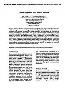
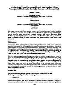
In a building, the central chiller plant has plenty operating parameters (variables) that can be controlled to minimize the running costs. At any given time, different combined modes of chiller operation and set points are possible to meet the instantaneous cooling demand. The part-load performance of a chiller depends on the method by which its capacity is modulated. Chillers can be successfully operated as low as 30 to 40% of the nominal design flows. Figure 1 shows a circuit diagram of a chiller system. If fixed-speed pumps are selected and sized to give proper flows to a chiller at design conditions, then they are oversized for part-load conditions and the system will have higher operating costs than with variable-speed pumps having the same design capacities. [Waltz 2000] Nevertheless, the power requirements are similar at running conditions close to the peak loads, during which the speeds under variablespeed control approach those of the fixed-speed operation. Hence the overall savings over a cooling season associated with the use of variablespeed equipment depends upon the building load profile.
cooling water loop T4, m2
T3, m2 cooling water pump
Water-cooled condenser refrigerant loop
Chiller
Evaporator
T2, m1
T1, m1 chilled water pump
chilled water loop Air-handlers with Qc
Fig.1 Chiller system for HVAC application
- 1059 -
can also be modified to facilitate the application of tri-generation or combined cooling, heating and power (CCHP). The technique recovers the exhaust heat of power generator as the fuel input to the chiller, resulting in dramatic energy saving. Absorption technology operates with no ozonedepleting CFC and hence causes less global environmental problems.
SYSTEM OPTIMAL CONTROL Optimal control of a chiller system asks for minimizing the total power consumption of the system components at each instant of time, with respect to the independent continuous and discrete control variables. Examples of the independent continuous control variables are set temperatures of chilled/cooling water, relative water flow rates to multiple chillers (at both evaporators and condensers), pump and fan speeds, etc. Discrete control variables are not continuously adjustable, but have discrete settings, for instance the number of operating chillers, fans and pumps. In addition to the independent optimization control variables, there are also local loop (dependent) controls associated with the chillers, pumps, air handlers, etc. The optimal control variables change through time in response to uncontrolled variables. The uncontrolled variables are measurable quantities that may not be controlled but that affect the component outputs and costs, such as the load and ambient dry-bulb and wet-bulb temperatures. Component-based optimization methodology is very often utilized as a tool for investigating chilled water systems. With this tool, general guidelines are incorporated in the system-based near-optimal control methodology.
Fuel energy plus electricity consumption represents an important factor in evaluating the overall performance of an absorption chiller system. In modern design, variable speed pumps are used. Good control strategy is an effective way to maximize the chiller system performance. To characterize the chiller quantitatively, one typically measures COP and the instantaneous load Qc at assorted values of coolant inlet temperatures.
For a given system, the best solution for determining the optimal control is to have a detailed model of the complete process that operates in parallel with an actual system. An optimization algorithm is then applied to this model. However, this type of approach requires detailed measurements for each system component in order to update parameters of the models so that they adequately match the real performance. Often these measurements are either not available or inaccurate. In addition, the description of the system to be modeled and optimized requires considerable expertise. As a matter of fact, all dynamic thermal models are approximations; it is the mathematical background that makes them different.
Fig.2 Direct-fired double-effect LiBr absorption chiller The absorption chiller itself is a complicated nonlinear system. In order to work out the mathematical model of the absorption chiller system, many research efforts were spent on analyzing the system physical behavior, such as the works of Grossman and Michelson [1985], Grossman and Gommed [1987], Gommed and Grossman [1990], also Hellmann and Zieglar [1999]. Component models have been built upon a number of governing equations, including energy balance, conservation of total mass, conservation of absorbent, heat transfer, thermodynamic equilibrium between liquid and vapor, etc. The component models contain complex thermodynamic equations with a series of assumptions. The nonlinear structure of these equations often prevents the development of reliable converging solution modules. Moreover, the functional relations are mainly expressed in terms of the chiller physical characteristics such as heat transfer coefficient-surface area (UA), concentration of absorbent at every state points,
ABSORPTION CHILLER SYSTEM Figure 2 shows a direct-fired double-effect LiBr absorption chiller. A direct-fired absorption chiller system adopts a more direct energy conversion cycle than a vapor-compression chiller. It incurs more heat rejection than a vapor-compression one of similar capacity. The system uses the heat input for one de-absorption effect, and the warm refrigerant vapor for another de-absorption effect. The condenser, evaporator and expansion device of an absorption chiller perform relatively the same functions as those in vapor compression systems. The system is able to provide space cooling, heating and hot water supply simultaneously. It
- 1060 -
etc. These kinds of technical information must be obtained or deduced from the manufacturer data in one way or the other. Detailed measurements at every system components are required in order to update the model parameters, so that they are adequately matching the real life parameters. A complete data set is nearly impossible to get [Braun et al. 1989]. In system optimization however, the users and the system designers are interested only in some of the system states (variables), and not every states of the entire chiller system. At this end, artificial neural network (ANN) is a technique which concentrates on describing the system inputs-outputs relationship, and is highly useful to predict the system behavior without tracing hard the underlying physical laws.
Input u1
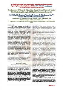
ANN represents a non-algorithmic, black-box computational strategy. It is composed of interconnected artificial neurons; each has an input/output (I/O) characteristic and implements a local computation. Figure 3 shows an artificial neuron with r number of inputs. A weight w is assigned to each input u to describe its influence (strength). The sum of the weighed inputs and the bias b forms the input to the activation function f, which can be either linear or nonlinear differentiable. The output a from the neuron is then given by
r a = f ∑ w1,i u i + b i =1
w1,1
u3
. . w1,r
Σ
n
f
(1)
The mutilayer feedforward (FF) network structure, as in Figure 4, is so far one of the most popular and effective ANN structure. Here the first (input) layer Li serves as a holding site for the inputs. The last (output) layer Lo is the point at which the overall mapping of the network input is available. In between these two are the hidden layers Lhi, where additional re-mapping, or computing takes place. Each layer, based on its inputs, computes output vector and propagates this information to the succeeding layer.
General Neural
u2
ur
ANN SIMULATION
a
b 1
Thus the FF network allows parallelism (parallel processing) within each layer, though the flow of interlayer information is necessarily serial. Its mathematical operation can be seen as the superposition and composition of nonlinear functions. The choice of a black-box structure still requires several ANN design considerations, i.e.
a=f(wu+b)
Fig.3 Neural model
Fig.4 Multilayer feedforward network structure
- 1061 -
the topology of the internal network, the characteristics of the internal units, the appropriate formulation of inputs/outputs, the design of training or learning procedures.
where a is the mean value of all actual outputs. The ANN model can be regarded as a good representation of the system if the R values of all output variables are small, say less than 0.1.
Neural network can be described as a machinelearning technique. Modifying the numerical values of its connection weights through certain training algorithm causes the network to approach the solution of a system model. Numerous researchers under different constraints have shown that multi-layer FF ANNs are capable of approximating any finite function to any degree of accuracy [Hornik et al. 1989, Cotter 1990]. The learning ability of a neural network depends on the arbitrary choices of its architecture as well as the training algorithm. The choice of activation function may significantly influence the applicability of a training algorithm. Lack of success in applications is likely attributable to faulty training, faulty architecture (incorrect numbers of hidden units), or lack of a functional relationship between inputs and outputs [Schalkoff 1997].
The main objective in ANN design and training is to produce networks that are able to apply correctly to new unforeseen inputs. By partitioning the available data sets, some testing sets are reserved for assessing the generalization performance. This is known as cross validation. Over-training might lead to memorization, and therefore poor performance when applying the testing sets.
1. 2. 3. 4.
ANN computation input (u)
One of the biggest shortcomings of FF network is the limited availability of suitable training algorithms. So far back propagation (BP) has been found highly successful [Hagan et al., 1996]. The standard BP algorithm is a gradient descent algorithm, which adopts an error correction-based learning procedure. The Levenberg-Marquardt (LM) algorithm is an alternative method for achieving fast optimization.
1 n ∑ (t i − ai ) 2 n i =1
(2)
where ai refers to the normalized actual (neural network) output values corresponding to “n” number of sets of independent input variables, and ti is the normalized target (real) output values for the same sets of input variables. For any output variable during a simulation process, its correlation coefficient R, that compares the complete set of actual outputs with the targets, is an indicator of how well the targets can be explained by the actual outputs. By definition,
R=
1 a
1 n (t i − ai ) 2 ∑ n i =1
network parameters revision (wij, b) Training procedure training set
Fig.5 Multilayer FF supervised training process
ILLUSTRATION
In the process, the performance of the network can be evaluated by the mean square error (MSE), which is defined as:
MSE =
output (a)
(3)
- 1062 -
A chiller system with the use of a direct-fired double-effect LiBr absorption chiller having a nominal rated cooling capacity of 989 kW (280 refrigeration tons) had been investigated by the mentioned ANN approach. Figure 5 shows an ANN training example of this absorption chiller system – one with 4 layers and having 5 input variables and 4 output variables. The selection of inputs and outputs depends on the real application/representation of the system model. In this chiller case the model was used for finding the best combination of chilled water and cooling water flow rates and temperature settings in order to minimize the overall energy cost of the plant at various cooling loads. The cooling tower fan operation was not a subject of our study since in Hong Kong the use of evaporative cooling devices has been forbidden in commercial chiller application for some years, owing to the scarcity in water resource. The inputs therefore included 4 independent control variables: the set point temperature of chilled water supply (T2), the chilled and cooling water mass flow rates (m1, m2), the return cooling water temperature (T4), plus an
layers, testing had been carried out for various numbers of nodes up to 15 per layer. In all these configurations, the networks were fully connected. Tan-sigmoid transfer function was used as the activation function for the hidden layers, and linear transfer function was used for the output layer. The LM algorithm was applied until finally the evaluation standard was reached. In the trainingby-epoch process, cross-validation was used and error trajectories were monitored. The auto-stop function was imposed. It was found that all ANN architecture with single hidden layer could not achieve in satisfactory results. Their MSE values were all greater than 0.01 and the R values for Pcool were greater than 0.18, and hence indicating poor prediction accuracy. Acceptable results were obtained for 19 cases of 2 hidden layer configurations, in which MSE < 0.01 and all R values < 0.1. The implication was that the error of prediction would not be higher than 10% in these cases.
uncontrolled variable: the cooling load (Qc). Oil consumption and water pump power are the primary contributors of energy cost in this system, whereas the chiller coefficient of performance (COP) reflects accurately the system efficiency. Therefore, the outputs included the mass flow rate of diesel oil (Mfuel), the respective electric power of the cooling water pump (Pcool) and the chilled water pump (Pchill), and the COP. The operation of an absorption chiller system has to be limited to certain ranges of operating parameters to guard against solution crystallization and evaporator freezing problems. To ensure a good representation of the test data in the current study, field measurements of the chiller system were taken under a wide range of load conditions from 30% to 120%. 2,100 sets of test data were finally used through a mix of field measured and catalogue deduced data. The numerical values of the test data were normalized to within the range of -1 to 1.
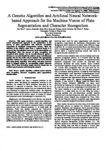
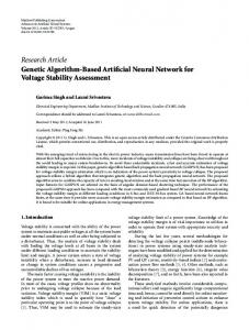
The configuration 5-5-9-4 came out to be the most optimal topology. The training process stopped at 450 iterations and the MSE value was 0.00285. The corresponding R values were 0.0494 for COP,
The training was executed systematically over a family of architectures, including both single- and two- hidden-layer configurations. For the hidden
a
a
t (Mfuel)
t (COP)
a
a
t (Pchilled)
t (Pcool)
Fig.6 The plot of actual outputs against ANN outputs for 5-5-9-4 configuration
- 1063 -
While the fitness requirements are being updated from time to time, a new generation of the population will be produced using the three genetic operators: selection, crossover and mutation. [Haupt and Haupt 1998] The new generation will go through the same evaluation process. This cyclic process continues until the maximum number of generations has been reached. The final population of the generation groups is designated the "winner" and rewarded the final generation of lowest cost (final fitness).
0.0564 for Mfuel, 0.0804 for Pcool and 0.0724 for Pchilled respectively. The plots of target outputs (t) against actual outputs (a) are given in Figure 6. It can be seen that the data points are distributed close to the best linear fit of a = t.
GA APPLICATION The association of GA with ANN was found highly appropriate applying to this chiller system control optimization study. Their advantages can then be made full use of, i.e. the ability of ANN to learn complex nonlinear mapping [So et al. 1995], and that of GA to find the global optimum in a bounded parametric search space [Asiedu et al. 2000].
Start
Genetic algorithm is a general purpose, populationbased search algorithm in which the individuals in the population represent samples from the set of all possibilities. It allows the population to evolve under specified selection rules to a state that maximizes the “fitness”, which in this case is to minimize the cost function. Over time, the individuals evolve into even better individuals by sharing and mixing their information about the space. This is different from the point-based search methods, in which only a single point is evaluated at one time, and the next point to be evaluated is based solely on the evaluation of the previous point. In GA, the evolution is based on two simple concepts of natural evolution: “survival of the fittest” and “reproduction”. At each time step, called a generation, the individuals are evaluated and the fitter ones are selected to survive and produce offspring. The reproduction phase includes an operation in which two individuals can combine portions of their structures with each other, in an attempt to form “better” individuals in the next generation.
Input
Create initial random population
Perform ANN simulation
Evaluate GA fitness (cost) function Yes Is the stopping criterion satisfied? No Create intermediate population While (number of members in new population) < (population size) Do
Select two members at random
Figure 7 gives a brief outline of the optimization plan proposed for this study. The process begins with the identification of the system input variables and their constraints. The next step involves the development of the GA population of the input variables for use in the probabilistic-based optimum search. This is followed by the prediction of the system outputs based on the derived ANN model of the system. Once the outputs are available through the ANN computation, the relevant outputs are passed to the cost function routine to determine the latest values for comparison. The cost function Φ can be defined as the total energy cost rate in that:
Φ = C f Q f + Ce ( Pchiller + Pcool + Paux )
Final fitness
Perform crossover with probability Pc
Perform mutation with probability Pm
Insert members into new population
Fig.7 Brief outline of optimization plan
(4)
CONCLUSIONS
where Cf and Ce are the unit fuel cost and unit electicity cost, Qf is the fuel consumption rate, and Paux the auxiliary electric power.
Component-based optimization methodology is a popular tool to improve chiller system control but is not always the most successful one. In the case
- 1064 -
Haupt R.L. and S.E. Haupt, Practical Genetic Algorithms, John Wiley & Sons: New York, 1998.
of direct-fired absorption chiller system, the numerous assumptions behind the governing thermodynamic and fluid flow equations and the nonlinear structure of the equation set are the barriers to be overcome in numerical simulation for obtaining reliable meaningful solutions. A systembased ANN modeling approach can be an attractive alternative.
Hellmann H.M. and F.F. Ziegler, “Simple absorption heat pump modules for system simulation programs”, ASHRAE Transactions, Vol.105, Part 1, pp.780-787, 1999. Hornik K., M. Stinchcombe and H. White, “Multilayer feedforward networks are universal approximators”, Neural Networks, Vol.2, pp.359366, 1989.
The process of deriving an ANN model of a commercial absorption chiller system has been described in this paper. A practical integration of ANN with GA in achieving the final goal of minimizing operation cost is also suggested. To obtain a most matched but reasonably simple ANN configuration of the system model, a systematic search on the family of architecture is mandatory. Testing should be well monitored and crossvalidated. Adequate representation of the test data is a prerequisite for a successful outcome.
Schalkoff R.J., Artificial Neural McGraw-Hill: New York, 1997.
Networks,
So A.T.P., T.T. Chow, W.L. Chan and W.L. Tse, “A neural-network-based identifier/controller for modeling HVAC control”, ASHRAE Transactions, Vol.101, Part 2, pp.14-31, 1995. Song C.L., T.T. Chow, J.L. Chen and G.Q. Zhang, “ANN Identification Applying to Model Construction of the Direct-fired LiBr Absorption Chiller”, ACHRB 2000, IIR International Symposium, Shanghai, China, pp.258-263, Oct 2000.
ACKNOWLEDGEMENT This research project was supported by the Strategic Research Grant No. 7000971 from the City University of Hong Kong.
REFERENCES Asiedu Y., R.W. Besant and P. Gu, “HVAC duct system design using genetic algorithms”, HVAC&R Research, Vol.6, No.2, pp.149-173, 2000.
Waltz J.P., “Variable flow chilled water or how I learned to love my VFD”, Energy Engineering, Vol.97, No.6, pp.5-32, 2000.
Braun J.E., S.A. Klein, W.A. Beckman and J.W. Mitchell, “Methodologies for optimal control of chilled-water systems without storage”, ASHRAE Transactions, Vol. 95, Part 1, pp.652-662, 1989.
NOMENCLATURE a b COP Ce Cf f L Mfuel MSE m Pc Pchiller Pcool Pm Qc Qf R r T t u w
Cotter N.E., “The Stone-Weierstrass theorem and its application to neural networks”, IEEE Transactions on Neural Networks, Vol.1, No.4, pp.290-295, 1990. Gommed K. and G. Grossman, “Performance analysis of staged absorption heat pumps: waterlithium bromide systems”, ASHRAE Transactions, Vol. 96, Part 1, pp.1590-1598, 1990. Grossman G. and E. Michelson, “A modular computer simulation of absorption systems”, ASHRAE Transactions, Vol.91, Part 2B, pp.18081827, 1985. Grossman G. and K. Gommed, “A computer model for simulation of absorption systems in flexible and modular form”, ASHRAE Transactions, Vol.93, Part 2, pp.2389-2428, 1987.
Φ
Hagan M.T., H.B. Demuth and M. Beale, Neural network design, PWS: Boston, 1996.
- 1065 -
= actual output = bias = coefficient of performance = unit electricity cost ($/kWh) = unit fuel cost ($/kg) = activation function = layer = fuel consumption rate (kg/h) = mean square error = water mass flow rate (kg/s) = probability of crossover = chilled water pump electric power (kW) = cooling water pump electric power (kW) = probability of mutate = cooling load (kW) = fuel consumption rate (kg/h) = correlation coefficient = number of inputs = temperature (oC) = target output = input = weight = total energy cost rate ($/h)
- 1066 -