The 2010 IEEE/RSJ International Conference on Intelligent Robots and Systems October 18-22, 2010, Taipei, Taiwan
Approaches and Databases for Online Calibration of Binaural Sound Localization for Robotic Heads Holger Finger Institute of Neuroinformatics University of Zurich and ETH Zurich CH-8057 Zurich, Switzerland
Paul Ruvolo Machine Perception Lab University of California San Diego San Diego, CA 92093, USA
[email protected]
[email protected]
Shih-Chii Liu Institute of Neuroinformatics University of Zurich and ETH Zurich CH-8057 Zurich, Switzerland
Javier R. Movellan Machine Perception Lab University of California San Diego San Diego, CA 92093, USA
[email protected]
[email protected]
Abstract— In this paper, we evaluate adaptive sound localization algorithms for robotic heads. To this end we built a 3 degree-of-freedom head with two microphones encased in artificial pinnae (outer ears). The geometry of the head and pinnae induce temporal differences in the sound recorded at each microphone. These differences change with the frequency of the sound, location of the sound, and orientation of the robot in a complex manner. To learn the relationship between these auditory differences and the location of a sound source, we applied machine learning methods to a database of different audio source locations and robot head orientations. Our approach achieves a mean error of 2.5 degrees for azimuth and 11 degrees for elevation for estimating the position of an audio source. The impressive results highlight the benefits of a two-stage regression model to make use of the properties of the artificial pinnae for elevation estimation. In this work, the algorithms were trained using ground truth data provided by a motion capture system. We are currently generalizing the approach so that the training signal is provided online based on a real-time face detection and speech detection system.
Freund [5] use regression rather than classification to learn the mapping between sound features (in this case temporal delays between pairs of microphones in a microphone array) and servo positions that will drive the camera to look at the center of a sound source given a database of training samples. Saxena and Ng [3] compute the incident angle of audio using a single microphone equipped with an artificial pinna by exploiting the pinna’s direction specific modulation of the sound signal. In this approach, the learning process proceeds by estimating the statistics of likely sounds at various spatial locations using training data and then performing probabilistic inference (in this case using a Hidden-Markov Model) at test time. Machine learning approaches typically proceed in two phases. In the first phase, a database consisting of both recordings from a set of microphones (either mounted on a robotic head or in a microphone array) and the location of sound sources is collected for a period of time. In the second phase, this database is used as training data to some machine learning procedure to estimate the mapping between audio features and spatial location. While a number of studies[3], [4], [5] have shown that these approaches work well for robots that operate in dynamic environments, it is unclear that the models learned in one condition will generalize to new acoustic environments. Thus, it is important for robotic systems to adapt to changing acoustic conditions by continually collecting new statistics of the auditory-spatial map and adjusting location estimates accordingly. This is a significant challenge for existing machine learning algorithms for audio localization that assume a well-labeled set of training data for learning the localization map. In real world situations, it is unlikely that precise estimates of the location of sound sources will always be available. Adapting to changing acoustic conditions without the need for ground truth requires another sensor (e.g. a face detector) that is capable of estimating the position of sound sources in a room. Over time these noisy estimates of source location
I. INTRODUCTION Sound localization is fundamentally important in a number of subfields of robotics. For example, surveillance robots may orient towards areas of auditory activity and social interactive robots may turn towards a person that is addressing them. Traditional approaches to the problem estimate time delays between pairs of microphones and then use basic geometry to reconstruct the most likely location of the sound source [1]. While traditional algorithms based on computing temporal delays work well in laboratory conditions they tend to breakdown in real world settings [2]. Variability due to background noise and reverberant rooms can severely degrade the performance of these traditional algorithms. In recent years there has been an emerging literature focused on the application of machine learning approaches to sound localization [3], [2], [4], [5]. Ben-Reuven and Singer [2] formulate one-dimensional sound localization by discretizing the space of possible source locations and reducing the problem to multi-category classification. Ettinger and
978-1-4244-6676-4/10/$25.00 ©2010 IEEE
4340
can be combined with current measurements of auditory features so as to refine the mapping between auditory features and locations in space. To investigate these issues, we collected two datasets which we will make publicly available so as to accelerate progress in this field of research. The first dataset consists of several hours of audio collected from microphones mounted on a robotic head and ground truth positions provided by a motion capture system. The second dataset consists of audio, video, and motion capture recordings from two people conversing with each other while moving freely around in a room. In this paper, we provide baseline performance values for learning to localize sound sources on the first dataset. II. METHODS We first consider the problem of learning to localize and orient toward sounds using a database with known locations of sound sources. We proceed by describing our robotic head and defining the underlying spatial coordinate system. Next, we give algorithms for estimating two auditory features that are related to the spatial position of sound sources: interaural time differences (sometimes also called time delay of arrival) and interaural intensity differences (sometimes also called interaural level differences). The final section describes how to combine these auditory features to estimate the origin of the sound. A. Robotic Head The robotic head was constructed from a small brick of high density styrofoam attached to a 3 degree-of-freedom neck. The neck was controlled using three Dynamixel RX64 servo motors. The head was fitted with two artificial pinnae, each housing a microphone (see Figure 1). The pinnae were fabricated using a 3D printer and attached tightly in order to soundproof the microphones and to guarantee that the arriving sound waves can only pass through the corresponding pinna. For the sound recordings a Tascam UA-1641 mixer board and heart shaped microphones from Audix were used. Furthermore a Logitech Quickcam Vision Pro was mounted on the head to record the scene in front of the robot.
B. Coordinate System In this work, we define space in a special spherical coordinate system consisting of two axes (see Figure 2). The X axis runs through the center of the artificial ears and the Z axis runs perpendicular to it and corresponds to the longitudinal axis of the robotic head. As seen in the figure, α and β are the angles from these two axes to the sound source direction, where 0 < α < π and 0 < β < π. These two angles result in two potential locations on the sphere where the sound may have originated, in our work we choose the one in the front of the head as the output. The other half of the sphere which is in the back of the head is not considered. The transformation to a standard spherical coordinate system can be computed using the sine formula for spherical trigonometry. By applying the formula to α and β, we get the following equation for the azimuth angle Φ in a standard spherical coordinate system: ! p sin(α)2 − sin(| π2 − β|)2 (1) Φ = π − arcsin sin(β) The angle β is the elevation. From now on, we refer to the angle α as the azimuth to make the text more readable (although α is not an azimuth in a strict mathematical sense). Furthermore these angles are defined in the head reference frame and the transformation to the room coordinate system can be determined using the actual orientation of the three joints of the neck. The skeletal structure of the head joints was measured with the motion capture data and the transformation between the head and the room coordinate systems was computed using homogenous coordinates. Source
Z
!
Ear
X
Fig. 2. The head coordinate system with the two angles α and β to describe the orientation of the sound source. The X axis is the tilt axis. The Z axis is the pan axis. The Y axis is the roll axis and is not shown in the figure. α is the angle between the tilt axis and the sound direction measured along a meridian connecting the two ears. β is the angle between the pan axis and the sound direction measured along a perpendicular vertical meridian.
C. Auditory Features Fig. 1. Left: The experimental 3 degree-of-freedom robotic head. Right: Detail of the design of the artificial pinna.
1) Interaural Time Difference: The interaural time difference (ITD) refers to the difference in time taken for a sound to arrive at each of the two microphones (time delay of arrival). The observed ITD depends on the location of the
4341
sound source in space relative to the head, the geometry of the pinna and head, and the acoustics of the room. Thus, the delay between the recorded signals at the 2 microphones makes it possible to draw conclusions about the angle α between the position of the sound source and the axis through the center of the ears. We estimated ITDs using the generalized cross correlation method. Generalized cross correlation uses a pre-whitening filter to estimate this delay between the two signals. For a detailed description of common filter types we refer to Knapp and Carter [6]. In this work the following filters were used and evaluated for the computation of the time delays: SCOT, ROTH, PHAT, CPS-M, HT. To estimate the azimuth location of the sound source, a non-linear ridge regression was used to train a model which maps the ITD values to α. The non-linearities were applied both at the input level (ITDs) and the output level (the orientation of the sound source relative to the head). Assuming a sound that is infinitely far away, the sound waves arrive in parallel at the two pinnae. From this scenario, the mapping between the interaural time difference and the estimated angle α ˜ is given by α ˜ ≈ cos−1 (ITD)
(2)
where the distance between the head and the sound source is much greater than the distance between the two ears. After this non-linear transformation was applied to the ITDs and a new ridge regression model was trained, the results showed that this approximation would lead to a mapping which diverges at the edges. Without this cosine transformation, the mapping also diverges at the edges, but into the opposite direction. Consequently, the optimal solution must be a combination of both approaches. Instead of Eq. 2, we used the following linear combination with a weighting factor w: 2˜ α ) (3) π where 0 < w < 1. In our evaluation experiments described in Section III, we found the best results using w = 0.5. We used this value in all consecutive measurements. After this non-linear transformation the angle α is estimated using a regression with α ˜ as the input. In work not described here, interaural time differences were estimated from the outputs of a spiking binaural silicon cochlea [7] using the same database recordings. This hardware device uses the sound as input and generates spikes analogous to the biological cochlea. This new algorithm which uses the cochlea spikes to estimate the interaural time differences will be published separately. The output spikes of the silicon cochlea in response to the database recordings will also be publicly available. 2) Interaural Intensity Difference: Another source of information for sound localization is the difference in the intensity of the sound as it arrives at the two ears. This difference is typically known as Interaural Intensity Difference (IID). In general, the IID value depends on the frequency spectrum of the sound source, the orientation of the source with respect ITD ≈ w cos(˜ α) + (1 − w) · (1 −
to the head, the geometry and composition of the head and pinna, and the acoustic properties of the room. It has been shown [8] that humans use frequency specific modulations in IID to localize sound not only in the azimuth direction, but also in the elevation direction. However, for this feature to give usable information as to the location of sound sources the pinna must be constructed so that the frequency transfer function of the outer ear (pinna) depends on the direction from which the sound wave reaches the ear. The shape of the pinna is asymmetric and was chosen such that the interference caused by the reflecting sound waves depends on the elevation of the sound source location. Figure 1 shows the design of the artificial pinna used with our robotic head. The first step in computing the intensity difference was to calculate the Fourier transform of the sound signal at the left ear (Sl ) and at the right ear (Sr ). The interaural intensity difference for each frequency was computed using the equation IID(f ) =
Sl (f ) − Sr (f ) . Sl (f ) + Sr (f )
(4)
This formula effectively normalizes the intensity difference based on the total intensity in both channels. Due to the geometry of the pinna, these IID values are correlated with the elevation of the sound source location. In Figure 3, the blue and green curves show the correlations of the trials in which the sound location was on the left side (green) and the right side (blue) respectively. For the correlations shown in the upper figure only data points were used which were recorded with an angle α in the range from 70 to 90 (green) and 90 to 110 (blue) degree. The lower plot shows the datapoints which were recorded with an angle α in the range from 40 to 60 (green) and 120 to 140 (blue) degree. Within these ranges the angles α and β are randomly distributed. It can be seen that some frequencies are attenuated and others are amplified. Furthermore a comparison of the top and bottom figures shows that the average absolute value of the correlations are higher when α is such that the direction to the sound source is further on one of the sides of the head. The database used to construct this figure is described in detail in Section III. The corresponding pairs of correlation curves are roughly anticorrelated, which is expected due to the fact that the formula for the IID computation is antisymmetric with respect to a swap of the sides. This can be seen further in Figure 4 which shows the correlation between the curves in Figure 3 but for all possible variations of the angle α. It can be seen, that there is a strong correlation between neighboring regions (in red) and that there is a strong anticorrelation between regions with the same angle to opposite sides of the head (in blue). D. Estimation of Sound Direction In this section, we show how we combine the ITD and IID features to estimate the azimuth and elevation of the sound source. First, the input signals are separated into small windows. Then the generalized cross correlation method is
4342
α = 70−90 degree and 90−110 degree 1 α = angle between pitch axis and sound source
0.8 0.6 Correlation between IID and β
1
0
sound left sound right
0.4 0.2 0 −0.2 −0.4 −0.6
0.8
20
0.6 40 0.4 60 0.2 80 0 100 −0.2 120 −0.4 140 −0.6
−0.8 160 −1
0
10
20
30
40 50 60 Fourier Component
70
80
90
0
100
20 40 60 80 100 120 140 α = angle between pitch axis and sound source
160
α = 40−60 degree and 120−140 degree
Fig. 4. Correlations between the curves shown in Fig. 3 for all combinations of α values.
1 sound left sound right
0.8
Correlation between IID and β
0.6
estimate the elevation β within this bin. In our evaluations we used a bin size of 10 degree to discretize α, which means that we trained 18 different linear models to estimate β. This 2-stage regression with the selection of the second regression model depending on the output of a first regression is another non-linearity in the system. In future work the bin size should be further invesitgated. There are also piecewise linear predictor models that automatically divide a non-linear problem into several linear problems as shown by Hartono [9]. In the end, the values of α and β are transformed to spherical coordinates using Equation 1. An overview of our localization algorithm is shown in Figure 5.
0.4 0.2 0 −0.2 −0.4 −0.6 −0.8 −1
0
10
20
30
40 50 60 Fourier Component
70
80
90
100
Fig. 3. Correlations between the elevation and the interaural intensity differences in each frequency for specific ranges of α. In the upper figure, the green curve corresponds to an azimuth angle between 70 and 90 degree and the blue curve to an azimuth angle of 90 to 110 degree. In the lower figure, the green curve corresponds to an azimuth of 40 to 60 degree and the blue curve was measured at an azimuth angle of 120 to 140 degree. Within these ranges the angles α and β are randomly distributed.
used to estimate the interaural time differences which are used to estimate α using simple geometric relationships (Chapter II-C.1). Next, interaural intensity differences are computed separately for each Fourier component of the input signals (Chapter II-C.2). A ridge regression is then used to make a more precise estimate of α. The features for this ridge regression are the angles α ˜ computed with Eq. 3. This feature set was then extended with the IID values, which showed a small improvement in the performance to estimate the azimuth. But considering the increase in computation time and the small performance gain we did not pursue it further in the work in this document. Next we estimate β. As can be seen in Figure 3, the mapping between IID and β is heavily dependent on the value of α. Therefore we discretize the range of α and construct a different linear model for each discretized bin to
III. E VALUATION A. Database Collection Both datasets were recorded in a motion capture room with the size of approximately 8x8 m. The room was equipped with a PhaseSpace motion capture system with 24 Impulse cameras distributed around the room, which record the positions of LEDs that were mounted on the sound sources and on the robotic head sampled at 240 Hz. 1) Database with Loudspeaker: This first database was used for the evaluations presented in Section III-B. The database consists of recordings from two microphones inside the robotic head in response to a soundclip played through a loudspeaker which was placed at a distance of 2.5m away. There were 4 LEDs mounted on the robotic head so that its position and orientation can be computed using the motion capture data. Furthermore the position of the loudspeaker was measured with another LED. The loudspeaker was placed at one of three possible azimuth angles around the robotic head. At each azimuth angle, the loudspeaker was placed at one of two possible heights which are spaced 1 m apart. The two heights and three azimuth angles gives us a combination of six possible loudspeaker positions. For each of these six positions,
4343
3 Front Back 2.5
β
2
1.5
1
Non-Linear Transform: Eq. 2
0.5
0
0.5
1
1.5
2
2.5
3
3.5
α
Fig. 6. The angles α and β of the recorded data in the head coordinate system. The blue points are in the front of the head and the red points are in the back of the head. In the evaluation of our proposed sound localization algorithm, we used only the blue recording points.
Fig. 5. Flow diagram showing the proposed sound localization algorithm. The use of IID values for the ridge regression to estimate α (dashed line) showed only a small performance improvement so that it was not used in further evaluations.
recordings were collected for 125 different orientations of the robotic head. These 125 orientations were achieved by evenly dividing each of the three degrees of freedom of the neck into five positions. Together with the 6 possible positions of the loudspeaker, we collected recordings from 750 different sound source locations measured in the head reference frame. These recorded positions are shown in Figure 6. For each of these positions, a 26 second soundclip was played through the loudspeaker. The soundclips consist of 5 seconds of white noise, 5 seconds of female speech, 5 seconds of male speech, 5 seconds of female and male speech mixed, 5 seconds of a laughing child and 1 second to record the impulse response. The recordings over the 750 locations resulted in a total recording time of 325 minutes. 2) Database of Conversations with Visual Recordings: The second database consists of short segments of two people taking part in a conversation. A total of 3 subjects participated in 9 recording sessions, each around 3 minutes long. In 3 of recording sessions, the two subjects were instructed to look to the robotic head during the whole conversation. In 3 other sessions, the subjects were instructed to look at the other person that is taking part in the conversation. In the 3 remaining sessions, there was no clear instruction given and thus the subjects freely switched their orientations between the robotic head and the other person. Simultaneous with the audio recording, we also recorded video from a camera mounted in the middle of the robot’s head. The dataset presents a very challenging setting for machine learning approaches to audio localization. One
challenge is that the video data contains a large amount of motion blur due to the frequent reorientation of the robotic head. A second challenge is that the speakers were not stationary and did not always face the robot when speaking. To allow for the easy evaluation of the performance of a system on this database, we recorded ground truth data on the location of each of the subjects and the robotic head using the motion capture system. There were 4 LEDs mounted on each person and on the robot head so that the exact position and orientation can be extracted from the motion capture recordings. Additionally, there were microphones attached near the mouth of each person so that information is available when each person is talking. The robotic head was oriented using a simple control algorithm. The head changed its orientation after every second. The control paradigm for every movement was chosen depending on whether a sound was detected in the last second interval. The head oriented itself to a random location if there was previously no sound detected. When there was sound detected during the last interval, the pan axis was oriented such that the front of the head points towards the sound source location. At the same time the tilt axis was always oriented randomly. The third axis (roll axis) was always set to the same value so that the line between the two ears is horizontal. B. Results 1) Prediction of Azimuth: In Figure 7, the predicted azimuth angle α is plotted against the actual α angle which was measured with the motion capture system. The mean error in the prediction of α was 2.5 degrees. We also investigated the effect of the length of the sound intervals which were used to estimate the azimuth on the performance. In Figure 8, the length of the time intervals was varied and the resulting correlation is plotted. Note the accuracy of the system increased as the length of the interval
4344
3.5
3
3 2.5
2 2
predicted β [rad]
predicted α [rad]
2.5
1.5 1
1.5
1 0.5 0.5 0 −0.5
0
0.5
Fig. 7.
1
1.5 2 real α [rad]
2.5
3
0 0.5
3.5
The predicted α angle vs the ground truth α.
Fig. 9.
1 Correlation between α and the prediction of α
2
2.5
3
The predicted β angle vs the ground truth.
fashion. Designing models that work well for learning in this fashion is something we wish to investigate in the future. The high diversity of the different types of recording sensors in the second dataset allows for further investigation on approaches that look at combining several senses and creating a calibration map between the sensors. In future, we will evaluate the use of visual information using a face tracker and visual speech detectors which can provide information about whether a person is talking or not, and we will integrate this information into the model.
0.98 0.96 0.94 0.92 0.9 0.88 0.86
V. ACKNOWLEDGMENTS The motion caputre equipment used for this work was funded by ONR DURIP Award # N000140811114. Paul Ruvolo and Javier Movellan were partially funded by NSF Science of Learning Center grant SBE-0542013, and NSF IIS INT2-Large 0808767.
0.84 0.82 0
1.5 real β [rad]
increased.
0.8
1
0.2
0.4
0.6 0.8 Interval Length [s]
1
1.2
1.4
Fig. 8. Correlation between the predicted angle and the real angle for different sound intervals.
2) Prediction of Elevation: In Figure 9, the predicted elevation angle β is plotted against the real angle measured using the motion capture system. The mean error in the prediction of elevation was 11 degrees. IV. C ONCLUSION AND F UTURE W ORK In this work we presented a 2-stage algorithm that estimates the location of a sound source in azimuth and elevation based on a robotic head with artificial pinnae. An advantage of our system compared to stationary microphone arrays is that in our system microphones are attached directly to the head and thus it is possible for us to record from a mobile robot that can easily move between different rooms. In addition we wish to expand our coordinate system to include sound sources behind the robotic head as well as the distance to the sound sources. We also identified the problem of an online visually guided calibration of auditory localization as a logical next step for machine learning approaches to audio. A major contribution of this work is the collection of a challenging dataset that will allow for approaches to this problem to be tested in a standardized
R EFERENCES [1] M. Brandstein and D. Ward, Microphone arrays: signal processing techniques and applications, Springer Berlin, 2001. [2] E. Ben-Reuven and Y. Singer, “Discriminative binaural sound localization”, Advances in Neural Information Processing Systems, pp. 1253– 1260, 2003. [3] Ashutosh Saxena and Andrew Y. Ng, “Learning sound location from a single microphone”, in ICRA’09: Proceedings of the 2009 IEEE international conference on Robotics and Automation, Piscataway, NJ, USA, 2009, pp. 4310–4315, IEEE Press. [4] K.W. Wilson and T. Darrell, “Learning a precedence effect-like weighting function for the generalized cross-correlation framework”, IEEE Transactions on Speech and Audio Processing, 2006. [5] E. Ettinger and Y. Freund, “Coordinate-free calibration of an acoustically driven camera pointing system”, in Distributed Smart Cameras, 2008. ICDSC 2008. Second ACM/IEEE International Conference on, 2008, pp. 1–9. [6] CH Knapp and GC Carter, “The generalized correlation method for estimation of time delay”, IEEE Transactions on Acoustics Speech and Signal Processing, vol. 24, no. 4, pp. 320–327, 1976. [7] Minch B Liu S-C, van Schaik A and Delbruck T, “Event-based 64channel binaural silicon cochlea with Q enhancement mechanisms”, IEEE International Symposium on Circuits and Systems, 2010. [8] J.C. Middlebrooks and D.M. Green, “Sound localization by human listeners”, Annual Review of Psychology, vol. 42, no. 1, pp. 135–159, 1991. [9] P. Hartono, “Ensemble of linear experts as an interpretable piecewiselinear classifier”, Innovative Computing, Information and Control Express Letters, vol. 2, no. 3, pp. 295–303, 2008.
4345