Approximate parameter inference in a stochastic reaction-diffusion ...

Approximate parameter inference in a stochastic reaction-diffusion model

Andreas Ruttor TU Berlin, Germany

Abstract

Manfred Opper TU Berlin, Germany

Statistical inference for such processes is highly nontrivial because

We present an approximate inference approach to parameter estimation in a spatio-temporal stochastic process of the reaction-diffusion type. The continuous space limit of an inference method for Markov jump processes leads to an approximation which is related to a spatial Gaussian process. An efficient solution in feature space using a Fourier basis is applied to inference on simulational data.

1

• observations are not independent but are generated from a Markov process with continuous time. • Space is continuous. It is not clear if an inference method for a spatially discretized model remains computationally tractable when discretization becomes finer and finer. • Fluctuations may not be irrelevant: The transition to a spatial continuum limit is often enabled in the limit where the number of molecules is large enough to safely neglect density fluctuations. The evolution of the macroscopic density is then typically governed by a partial differential equation (PDE). In some cases it is possible to solve the PDE for the stationary (time independent) density analytically which could be used as a fit to experiments. However, neglecting the temporal dynamics usually does not allow us to estimate all rate parameters, but only certain ratios. Furthermore, measurements are often indirect and allow to estimate molecule densities only up to an unknown scale factor. Then even a time dependent solution of the macroscopic PDEs would not be sufficient to infer those parameters which directly determine molecule numbers (such as creation rates) and the stochasticity of the spatio-temporal process must be discussed. For the relevance of fluctuations in the biological context, see (Tostevin et al., 2007).

Introduction

Reaction-diffusion models are used to describe spatio-temporal stochastic processes where molecules diffuse through space, are created and destroyed, and can participate in chemical reactions when they are close. This type of process finds a variety of applications in chemistry, physics (Gardiner, 1996), and also in the field of computational biology. Recently the propagation of the Bicoid protein, which is relevant for morphogenesis in the Drosophila embryo, has been modelled by such a process (Wu et al., 2007). In many applications, one can assume a qualitative knowledge of basic processes in the model. However, the numerical values of the parameters corresponding to these processes, such as the microscopic rates for diffusion, decay, and reactions, are often unknown. Hence, it is important to be able to infer such quantities from concrete experimental data. This is a problem of non-parametric statistical inference, because the natural description of the state of such systems is not in terms of the dynamics of individual molecules, but of the molecule density as a function of continuous space and time. Experiments typically provide (noisy) measurements of the (smoothed) molecule densities over a range of spatial locations at discrete times. Appearing in Proceedings of the 13th International Conference on Artificial Intelligence and Statistics (AISTATS) 2010, Chia Laguna Resort, Sardinia, Italy. Volume 9 of JMLR: W&CP 9. Copyright 2010 by the authors.

The problem of inference in continuous time Markov processes has recently attracted attention in the machine learning/AI community and a variety of approximate inference methods for these models have been developed (Archambeau et al., 2008; Cohn et al., 2009; Nodelman et al., 2005; Opper and Sanguinetti, 2008). However, it is not clear if these methods will scale up to be able to deal with the complexity of fluctuating spatial densities. In this paper we present an approach for approximate inference in a reaction-diffusion model which takes both Markov dynamics and spatial fluctuations into account. The method is based on a recently developed approximate inference method for Markov jump processes (Ruttor and

669

Approximate parameter inference in a stochastic reaction-diffusion model

Opper, 2009) which easily allows for the transition to a continuous space. We apply the method to a model which contains the basic processes relevant for the Bicoid protein evolution in Drosophila (i.e. creation and decay of molecules, but no chemical reactions between molecules), but uses a simplified one dimensional geometry. We have used this model as a proof of concept for our inference approach. The data sets were obtained from simulations of the model and the measurement process using realistic true system parameters (Wu et al., 2007). This allows us to see how well these parameters can be inferred from data. We have not yet applied the model to real measurements, because available data at different time points are taken from different embryos and are thus not based on the statistical assumptions of our model. Obtaining the more interesting in vivo measurements on a single embryo is nontrivial, but should hopefully be possible in the near future (Wu et al., 2007).

2

Reaction-diffusion models as Markov jump processes

A sound description of the stochastics of reaction-diffusion models can be based on a compartment model (Gardiner, 1996), where space is discretized into small cells of size ∆x (assuming a single space dimension for simplicity). The state of the system is described by a vector n = (n0 , . . . , nM ), where ni is the number of molecules in a cell. The stochastic dynamics is assumed to be a Markov jump process (MJP) defined by a rate function f (n′ |n) which determines the temporal change of transition probabilities via

P n′ ,t + ∆t|n,t ≃ δn′ ,n + ∆t f n′ |n (1)

for ∆t → 0. The rate f (n′ |n) is the sum of the rates for all individual processes which lead from n to n′ .

3

While it is not possible to perform exact inference on this model, we will resort to an approximate inference approach for Markov jump processes following the work of Ruttor and Opper (2009). The main contribution of the present paper is to extend this method to the non-parametric continuum limit required for reaction-diffusion models. Here the cell size ∆x shrinks to zero and molecule numbers ni are replaced by densities ρ (x) via ni → ρ (xi )∆x .

• In a similar way we can treat Molecule degradation n′i = ni − 1 which occurs with a rate λ ni in all cells. • Creation of molecules in the system occurs by injection with a fixed rate c/∆x in a single cell only.

(2)

We will next briefly review the main results of Ruttor and Opper (2009) needed for our application. Parameter inference of Markov jump processes can be based on the recursive computation of

ψ (n,t) ≡ P(D≥t |θ , n(t) = n) ,

(3)

the likelihood of future observations D≥t = {yi }ti ≥t conditioned on the state n(t) = n at the present time t. The likelihood of all data is used for maximum likelihood or Bayesian estimation of rate constants c, d, and λ is consequently p(D|c, d, λ ) = ∑ ψ (n, 0)p0 (n) , (4) n

where p0 (n) is the distribution of the initial state. For times between two observations ψ (n,t) obeys the Kolmogorov backward equation   d ψ (n,t) = ∑ f (n′ |n) ψ (n,t) − ψ (n′ ,t) , dt n′ 6=n

(5)

which has to be solved backward in time with the end condition ψ (n,tN ) = p(yN |n(tN )). The observations enter consecutively from the latest to the first one through their conditional distributions (assuming independent noise) p(y|n), in the jump conditions

In the Bicoid system we consider three types of elementary processes: • Particle diffusion, say from cell i into the neighboring cell i + 1, is modelled by a transition n′i = ni − 1 and n′i+1 = ni+1 + 1 with a rate d ni /∆x2 , where d is the diffusion constant of the system. The proportionality of the rate to the number ni of molecules accounts for the fact that each of the molecules can perform the jump to the neighboring cell. As we will show later, the factor 1/∆x2 will allow for a proper limit ∆x → 0 of the compartment model.

Approximate Inference for MJPs

lim ψ (n,t) = p(yl |n(tl )) lim ψ (x,t) ,

t→tl−

t→tl+

(6)

where tl− and tl+ denote the left and right side limits. Similar to the backward-forward algorithm in Hidden Markov Models state inference at arbitrary times t can be performed using ψ (n,t) together with a solution of the (forward) master equation. The approximation method of Ruttor and Opper (2009) is an extension of van Kampen’s system size expansion approach (Gardiner, 1996; van Kampen, 1981) originally developed for solving the forward Master equation to the problem of statistical inference. Assuming systems with sufficiently large numbers of molecules, the state n of the system is essentially approximated by a vector with continuous components which have Gaussian fluctuations around a macroscopic state.

670

Andreas Ruttor, Manfred Opper

Formally, the system size expansion can be derived by a combination of a diffusion approximation to the Master equation together with a subsequent Gaussian ‘weak noise’ approximation, where small relative fluctuations are assumed. 1 Applying the same ideas to the Kolmogorov backward equation Ruttor and Opper (2009) derive an approximation to (5) by the partial differential equation

∂ ψ (n,t) + (n − b)⊤ A⊤ (b(t))∇ψ (n,t) ∂t 1 + Tr(D(b(t))∇∇⊤ )ψ (n,t) = 0 . (7) 2 Here b denotes the macroscopic state of the system for which fluctuations are ignored and ∇ is the vector of partial derivatives with respect to n. This fulfils the classical rate equation db = f(b) , (8) dt where f(n) = ∑ f (n′ |n)(n′ − n) (9) n′ 6=n

is the first jump moment or drift vector of the transition rates. The matrix A = ∇f⊤ is the Jacobian of the first jump moment. The diffusion matrix (again not to be confused with the diffusion constant d for the molecules) D(n) =

(n′ − n) f (n′ |n)(n′ − n)⊤ ∑ ′

(10)

n 6=n

is defined by the second jump moments. The dependency of D(b) on b accounts for the fact that fluctuations depend on the number of molecules. Eq. (7) is the backward equation for a Gaussian diffusion process of the Ornstein-Uhlenbeck type (Gardiner, 1996). For observations with Gaussian noise, it can be shown that the solution ψ (n,t) of (7) is of the form   1 z(t) ψ ≈ 1/2 exp − (n − b(t))⊤ S−1 (t)(n − b(t)) . (11) 2 |S| Although ψ (n,t) (as a solution to a backward equation) is not a normalized probability, we will refer to (11) as a Gaussian. This analogy is helpful when we later apply linear transformations such as Fourier transforms to the variables. Between observations the dynamics of b(t) is given by (8) and the matrix S(t) and normalizer z(t) evolve according to the ODEs dS = AS + SA⊤ − D(b) , (12) dt dz = z(t) Tr(A) . (13) dt 1 Note,

that the term diffusion here refers to the stochastic dynamics of the vector n and should not be confused with the diffusion of the molecules.

The end condition for S is given by S(tN ) = σ 2 I in the case of independent Gaussian measurement noise with standard deviation σ . Here I denotes the unit matrix. Using the rates of the MJPs for the compartment model, assuming that molecules are created at site i = 0 only, one can derive the following expressions from (9) and (10) for drift vector and diffusion matrix: d (ni+1 + ni−1 − 2ni ) fi (n) = ∆x2 − λ ni + c δi,0 d (ni + ni+1 )(δi, j − δi+1, j ) Di, j (n) = ∆x2 d (ni + ni−1 )(δi, j − δi−1, j ) + ∆x2

(14)

+ δi, j λ ni + δi,0 δ j,0 c .

(15)

Here δi, j denotes the Kronecker symbol which equals 1 for i = j and 0 else. In spatially homogeneous reaction systems both drift vector f and diffusion matrix D only depend on the state of the system and the reaction constants. But here, in the case of a compartment model for a reaction-diffusion system, there is an additional parameter to choose: the cell size ∆x. Of course, all information contained in the observations should be used by the inference algorithm. For that purpose ∆x has to be smaller than or at least equal to the spatial distance between two adjacent data points yi, j . However, shrinking the size of the compartments increases their number and the dimension of the matrices used in the calculation of the likelihood. Consequently, fulfilling this condition on ∆x is often not possible because of limited computational resources.

4

Continuum limit

A better way to solve this problem is calculating drift vector f and diffusion matrix D in the limit ∆x → 0 analytically. By doing so, we obtain a representation of the Bicoid model which decouples the effective dimension of the system state used in numerical calculations from the number of spatial components found in each observation yi . To perform the continuum limit we introduce the spatial positions xi = i∆x and particle densities via ρ (xi ) = ni ∆x. Denoting the macroscopic density corresponding to n by ρ¯ it is straightforward to perform this limit for the macroscopic rate equation (8). Using a Taylor series expansion to 2nd order around xi one obtains the well known classical diffusion equation

∂ ∂2 ρ¯ (x,t) = d · 2 ρ¯ (x,t) − λ ρ¯ (x,t) + cδ (x) (16) ∂t ∂x for molecules, which include the decay and a source term at x = 0, where δ (x) is Dirac’s δ distribution.

671

Approximate parameter inference in a stochastic reaction-diffusion model

To include density fluctuations in the continuum limit a useful strategy would seem to replace the multivariate Gaussian (11) for ni (t) by a corresponding spatial Gaussian process (Rasmussen and Williams, 2006) for the density ρ (x,t). The matrix S would then become a type of covariance operator. An explicit expression in terms of differential operators for this operator is indeed possible. Surprisingly, it is also possible to solve the operator differential equation corresponding to (12) analytically for our model. However, the subsequent computations of explicit operator inverses which are needed at the observations together with the normalizing determinant turn out be analytically intractable in position space. Hence, we have not pursued this route any further and give details elsewhere. It turns out that an equivalent approach to defining a Gaussian process in position space is to do that in a feature space (Rasmussen and Williams, 2006) where the fluctuating densities are expanded as an infinite linear combination of functions. The natural choice in our case is a Fourier basis for which a truncation with a relatively small number of features usually gives good results. The particle density of the molecules is expanded into a Fourier series, ∞

ρ (x,t) = ρ˜ 0 (t) + 2 ∑ ρ˜ k (t) cos(kπ x/L) ,

(17)

k=1

as well as the macroscopic density corresponding to n, ∞

ρ¯ (x,t) = ρˆ 0 (t) + 2 ∑ ρˆ k (t) cos(kπ x/L) .

(18)

k=1

Assuming reflecting boundary conditions at x = 0 and x = L the series can only contain cosine waves with frequencies kπ /L. In order to simplify further calculations we continue our model periodically in space with period 2L and symmetrically to x = 0, so that ρ (−x,t) = ρ (x,t). This is already a property of the Fourier series (17) and (18). Applying the Fourier transform to the classical diffusion equation (16) and taking the boundary conditions into account leads to # "   2 c k π + λ ρ˜ k + , (19) f˜k = − d L L which describes the drift f of the continuous model in Fourier space. It is possible to do a similar transformation for the diffusion operator D. But, in this case, a more elegant approach is to apply the discrete Fourier transform defined by

which results in   sπ   rπ 1 M M i∆x cos j∆x . D˜ r,s = 2 ∑ ∑ Di, j cos L i=0 j=0 L L

(21)

Afterwards we take the limit ∆x → 0, M → ∞ and arrive at      1 c rπ sπ ˜ Dr,s = 2d + λ ρ˜ |r−s| + 2 (22) 2L L L 2L for the diffusion D in the continuous model. In contrast to the corresponding equations (14) and (15) for the discrete compartment model, (19) and (22) do not contain the cell size ∆x. Then the solution ψ (ρ˜ ,t) of the backward equation in the Fourier representation is found to be   1 z(t) ψ ≈ 1/2 exp − (ρ˜ − ρˆ (t))⊤ S˜ −1 (t)(ρ˜ − ρˆ (t)) . (23) ˜ 2 |S| The Fourier representation of the densities has a remarkable property: Each component fk only depends linearly on the series coefficient ρ˜ k (t) for the same spatial frequency. Consequently, operator A is diagonal in Fourier space and the system of coupled matrix differential equations equations (8) and (12) for the compartment model becomes a set of uncoupled linear differential equations after applying Fourier transform and continuum limit: # "   d c kπ 2 ρˆk = − d + λ ρˆ k + , (24) dt L L # "    2 d ˜ rπ 2 sπ Sr,s = − d +d + 2λ S˜r,s dt L L      rπ sπ 1 2d + λ ρˆ |r−s| − 2L L L c . (25) − 2L2 All equations can be solved analytically in terms of exponential functions. Additionally, covariance components S˜r,s are only influenced by mean values ρˆk with k ≤ r and k ≤ s. Therefore it is possible to truncate all Fourier series at order N without affecting these calculations for lower frequencies at all. The only exception is the normalization factor z, because the likelihood of a Gaussian process depends on which features are actually observed: # "   N d kπ 2 (26) +λ . ln z = − ∑ d dt L k=0

(20)

However, as the right-hand side is independent of the system state, this dependency on N does not influence parameter estimation.

to the diffusion matrix of the discrete compartment model,

In summary, ψ (ρ˜ , 0) is calculated by integrating the ODEs (24), (25), (26) backwards in time and applying the jump

ρ˜ k =

1 L

M

∑ n j cos

j=0



kπ j∆x L



672

Andreas Ruttor, Manfred Opper

60

30 density stationary state

40

t = 240 t = 241 t = 242

20

ρ

y

20

10

0 0

50

100 x

150

0 0

200

50

100 x

150

200

Figure 1: Typical sample of the system after reaching the stationary state for parameters c = 30, d = 17.2, and λ = 0.027. The solid line shows the actual density of molecules, while the stationary solution of (16), the expectation value of the prior process, is given by the dashed line.

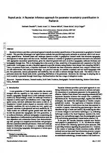
Figure 2: The first three observations of a data set as a function of position x. The data points were obtained from a simulation with parameters c = 30, d = 17.2, λ = 0.027, and noise level σ = 0.4 by convoluting the particle density with a triangle window of width l = 40.

condition (6) at each observation. Then the total likelihood is given by

the observations can be found in the low-order terms of the series expansion, while higher-order terms mostly contain noise and can be omitted in practise by truncating the Fourier series at order N. Note, that N can be smaller than M, which allows for a reduction of the computational complexity. We found that parameter estimation works well even if N is as small as M/2, which has been used to obtain the results shown in this paper. In contrast, the number of cells in the compartment model has to be greater than or equal to the number of spatial data points.

p(D|c, d, λ ) =

Z

ψ (ρ˜ , 0)p(ρ˜ 0 )dρ˜ ,

(27)

where p(ρ˜ 0 ) denotes the prior for the initial conditions. For the results shown here, we have used an uninformative prior, which is flat at observed lower frequencies, while it suppresses fluctuations at unobserved higher frequencies. In this special case we find p(D|c, d, λ ) ∝ z.

5

Observations

We also have to consider how observations are generated from the continuous density ρ (x,t). We assume that this measurement process for position xr and time ts can be described by a convolution of ρ (x,t) with a weight function w(x) in position space, yr,s =

Z L

−L

w(xr − x)ρ (x,ts ) dx + ξr,s

(28)

where ξr,s ∼ N (0, σ 2 ) denotes additive Gaussian white noise. This convolution corresponds to a product in Fourier space, so that each observed feature is just given as y˜k,s = w˜ k ρ˜ k (ts ) + ξ˜k,s .

(29)

We obtain M data points at positions xr = r L/M and use a triangle window of width l = 2L/M, so that the weights w˜ k in Fourier space are given by −2    2π 2π kl kl . (30) sin2 w˜ k = L L Here high frequencies are just averaged out in the measurement process. Therefore all information contained in

Our inference method can use other weight functions, too. This is especially useful if the characteristics of the real measurement process are known. As long as the measurement window is large compared to the spatial distance between adjacent observations, our algorithm works without modifications. But if a small window does not suppress high frequencies sufficiently, these are folded back into the low frequency components of y˜k,s by the discrete Fourier transform. In this case one has to replace ψ (ρ˜ ,t) with the ˜ ρ˜ ,t) for a weighted density. corresponding likelihood ψ (w

6

Simulations

Although real data from biochemical experiments is not yet available, we can generate observations using simulations of the model. For that purpose, we could use the Gillespie algorithm (Gillespie, 1992) applied to the compartment model, which is quite a standard approach for Markov jump processes in a discrete state space. But choosing a well suited compartment size ∆x is difficult. If it is large, we only have to deal with a small number of state variables. Transfer reactions between the compartments are rare events, as the diffusion rate is inverse proportional to ∆x2 . In this case the Gillespie algorithm works well, but the spatial resolution of the simulation is rather low. Of

673

50

0.05

40

0.04

30

0.03

p(c|D)

p(λ|D)

Approximate parameter inference in a stochastic reaction-diffusion model

20 10 0 0

0.02 0.01

0.01 0.02

0.03 λ

0.04

0.05

0 0

0.06

10

20

30 c

40

50

60

Figure 3: Marginal posterior averaged over 200 data sets for the decay constant. The vertical line shows the true parameter value λ = 0.027.

Figure 4: Marginal posterior averaged over 200 data sets for the production rate. The vertical line shows the true parameter value c = 30.

course, improving it is possible by just using a large number of compartments. But a small compartment size ∆x also leads to a very high frequency of transfer reactions. Therefore the average waiting time between reaction events is small and the Gillespie algorithm, which processes single reaction events, becomes very slow.

7

Simulating the molecular dynamics of a reaction-diffusion model directly instead of using the compartment approximation can be an alternative. By doing so, we avoid the discretization error caused by the finite compartment size ∆x. As the Bicoid model only contains first-order reactions, diffusion processes of single molecules do not influence each other and can be solved analytically. Therefore the new position x(t + ∆t) of a molecule starting at x(t) after a time span ∆t is given by x(t + ∆t) = x(t) + ε , where ε is a Gaussian distributed random number,  √  ε ∼ N 0, 2d∆t ,

(31)

In order to test our method we have generated 200 different data sets from simulations of the Bicoid reaction-diffusion system with the same parameters. The values of the parameters are biologically plausible and were taken from Wu et al. (2007). Each sample contained 11 × 11 observations with spatial distance δ x = 20, temporal distance δ t = 1 and noise level σ = 0.4. An example is shown in figure 2. For each data set we have calculated marginal posteriors for the vector of parameters θ = (c, d, λ ) from a Laplace approximation to the posterior density (35)

F(θ ) ≡ − ln (p(D|θ ) p(θ )) ,

(36)

Laplace’s approximation is given by − log p(θi |D) ≈ F(θi , θ\i∗ ) +C ∂ 2 F(θ , θ ) 1 i \i + log 2 ∂θ2

(32)

(33)

take the degradation into account. And production is simply simulated by adding new molecules to the system. The waiting time tw between two production events for single molecules is also exponentially distributed according to p(tw ) = c exp (−ctw ) .

p(θ |D) ∝ p(D|θ ) p(θ ) . Setting

√ with zero mean and standard deviation 2d∆t. Exponentially distributed life times τ for each molecule, p(τ ) = λ exp (−λ τ ) ,

Results

(34)

As this approach works well, we have used it to generate observations as input for our inference algorithm. Figure 1 shows a typical sample obtained from such a simulation. It is clearly visible that spatial fluctuations cannot be neglected in this case.

, (37)

θ =θ ∗

where θ ∗ denotes the most likely parameters, i.e. θ ∗ = arg minθ F(θ ), θ\i all parameters without θi , and p(D|θ ) is computed from (27) using our approximate inference approach. For the prior distribution p(θ ) we have chosen a product of Gaussian densities cut off at negative values, with standard deviations equal to half of and means at the true parameter values. This choice was mainly done for simplicity and may have caused the peaks, which appear in the marginal posteriors for very low parameter values. The results of averaging the posteriors over the data sets are shown in figures 3, 4 and 5. It is clearly visible, that the modes of the averaged marginal posteriors are good estimates of the rate constants.

674

Andreas Ruttor, Manfred Opper

1

p(γ|D)

p(d|D)

0.2

0.1

0 0

10

20 d

30

0.5

0 0

40

1

2 γ

3

4

Figure 5: Marginal posterior averaged over 200 data sets for the diffusion constant. The vertical line shows the true parameter value d = 17.2.

Figure 6: Marginal posterior for γ averaged over 100 rescaled data sets with reaction constants as before. The vertical line shows the true parameter value γ = 2.

8

Indirect measurements and the role of fluctuations

internal noise of the system into account. For that purpose, we just have to treat γ as additional parameter.

While our model uses the density ρ (x,t) of the molecules in order to describe the state of the reaction-diffusion system, this quantity is usually not directly observable in biochemical experiments. There the molecules are marked with fluorescent particles and one observes the intensity I(x,t) of the emitted light, which is proportional to the density of the molecules (Wu et al., 2007):

Figure 6 shows the preliminary result of estimating γ averaged over 100 rescaled data sets. Each set contained 21 × 6 observations with spatial distance δ x = 10, temporal distance δ t = 2 and noise level σ = 0.4 for the intensities. Here we have kept the parameter λ at its true value. It is clearly visible, that estimation of the number of molecules from intensity measurements is possible using our algorithm. However, the uncertainty for γ is large, which indicates that this is a more difficult inference task.

I(x,t) = ρ (x,t)/γ .

(38)

However, the constant of proportionality γ , which depends on the preparation of the experiment and other factors, is usually unknown. We can take these indirect measurements into account by substituting ρ (x,t) with γ I(x,t) in our model. In this case the production rate c for molecules is replaced by a production rate cI = c/γ for intensity. The other rate constants d and λ , which describe diffusion and degradation respectively, are not changed by rescaling the state variables, as these are first order reactions. Therefore it is not possible to estimate γ using only the deterministic part (16) of the dynamics. But the covariances of the state variables contained in S and likewise the diffusion matrix D(ρ˜ ) are rescaled by 1/γ 2 , which results in      rπ sπ 1 ˜ ˜ 2d + λ I˜|r−s| (DI (I))r,s = 2γ L L L cI + . (39) 2γ L2 ˜ is the inhomogeneity in the linear differential equaAs D tion (25), it determines the size of fluctuations around the stationary state, which scale proportional to 1/γ . Consequently, we can estimate γ , because our model takes the

9

Discussion and Outlook

We have developed an approximate inference approach to parameter estimation for a simple class of reaction-diffusion models. Simulations suggest that our method is capable of dealing efficiently with the limit of continuous space and with fluctuations in the density. While the type of elementary processes considered so far are relevant to the biological Bicoid system, the one dimensional spatial geometry might be a strong simplification. Working with a 3-dimensional box geometry would be still possible using our Fourier basis without conceptual changes. More realistic geometries could be treated by using other types of specialized feature functions that are adapted to the boundaries of the problem. Bessel functions, for example, are a suitable basis for circular boundaries. A more challenging problem is the inclusion of chemical reactions between molecules. Again this can be modelled within the compartment approach and the continuum limit can be taken. However, this will usually lead to nonlinear macroscopic rate equations. Fluctuations may be still approximated by Gaussians analogous to (23) and would also be tractable by a suitable feature space representation. However in this case, analytical solutions to the temporal dynamics are not to be expected and a numerical integra-

675

Approximate parameter inference in a stochastic reaction-diffusion model

tions of ODEs is required. But we expect to find only a weak coupling between features of different order. Then we can still work with a reasonably small number of features and the nonlinearity is not a serious problem.

U. C. T¨auber, M. Howard, and B. P. Vollmayr-Lee. Applications of field-theoretic renormalization group methods to reaction-diffusion problems. J. Phys. A: Math. Gen., 38(17):R79–R131, 2005.

Finally, it will be important to assess the validity of the assumption of Gaussian fluctuations in our approximation. One might think that the success of such an approximation in the limit of infinitely small cell sizes in the compartment model is totally counterintuitive. Small cells contain only few molecules (or none at all) and fluctuations within a cell would be far from being Gaussian. One should note however, that what we really use in the inference method are the fluctuations of the leading Fourier coefficients of the density. Those are obtained from spatial averages of densities modulated with trigonometric functions of long wavelengths. This averaging takes advantage of the smoothness of the density function ρ (x,t) and might make fluctuations indeed more Gaussian. We expect that a formal analysis of our assumptions together with corrections to the approximation could be obtained from a functional integral approach to inference in reaction-diffusion models using ideas similar to T¨auber et al. (2005).

F. Tostevin, P. Rein ten Wolde, and M. Howard. Fundamental limits to position determination by concentration gradients. PLoS Computational Biology, 3(4):e78, 2007. N. G. van Kampen. Stochastic Processes in Physics and Chemistry. North-Holland, 1981. Y. F. Wu, E. Myasnikova, and J. Reinitz. Master equation simulation analysis of immunostained bicoid morphogen gradient. BMC Systems Biology, 1:52, 2007.

References C. Archambeau, M. Opper, Y. Shen, D. Cornford, and J. Shawe-Taylor. Variational inference for diffusion processes. In J. C. Platt, D. Koller, Y. Singer, and S. Roweis, editors, Advances in Neural Information Processing Systems, volume 20, pages 17–24. MIT Press, Cambridge, MA, 2008. I. Cohn, T. El-hay, R. Kupferman, and N. Friedman. Mean field variational approximation for continuoustime bayesian networks. In Proc. Twenty Fifth Conf. on Uncertainty in Artificial Intelligence (UAI 09), 2009. C. W. Gardiner. Handbook of Stochastic Methods. Springer, Berlin, second edition, 1996. D. T. Gillespie. A rigorous derivation of the chemical master equation. Physica A, 188:404–425, 1992. U. Nodelman, D. Koller, and C. R. Shelton. Expectation propagation for continuous time bayesian networks. In Proceedings of the Twenty-first Conference on Uncertainty in AI (UAI), pages 431–440, 2005. M. Opper and G. Sanguinetti. Variational inference for markov jump processes. In J. C. Platt, D. Koller, Y. Singer, and S. Roweis, editors, Advances in Neural Information Processing Systems, volume 20, pages 1105– 1112. MIT Press, Cambridge, MA, 2008. C. E. Rasmussen and C. K. I. Williams. Gaussian Processes for Machine Learning. MIT Press, 2006. A. Ruttor and M. Opper. Efficient statistical inference for stochastic reaction processes. Phys. Rev. Lett., 103(23): 230601, 2009.

676