table to short-circuit multiple recomputations of the same subgoal. So Tabled. Prolog tries ... computations along that chain can safely be deleted. However with ...
Approximate Pruning in Tabled Logic Programming Lu´ıs F. Castro and David S. Warren Computer Science Dept SUNY at Stony Brook Fax: +1 (631) 632-8334 {luis,warren}@cs.stonybrook.edu�
Abstract. Pruning provides an important tool for control of nondeterminism in Prolog systems. Current Tabled Prolog systems improve Prolog’s evaluation strategy in several ways, but lack satisfactory support for pruning operations. In this paper we present an extension to the evaluation mechanism of Tabled Prolog to support pruning. This extension builds on the concept of demand to select tables to prune. In particular, we concentrate on systems based on SLG resolution. A once operator is described, which approximates demand-based pruning, providing for an efficient implementation in the XSB system.
1
Introduction
Prolog is a programming language in which the programmer uses Horn clauses to specify a computation. Prolog uses a backward chaining, goal-directed, demanddriven evaluation strategy that can give it an advantage over forward chaining systems in that it tries to derive only subgoals that are relevant to the main query goal. So it evaluates only those predicates which are necessary to derive the goal. However, its strategy does allow it to derive the same (necessary) subgoal many times, leading, for example, to unnecessary exponential behavior when recognizing some context-free languages. Tabled Prolog [14] improves on Prolog in that, in addition to deriving only what is necessary for the goal, it will derive such subgoals only once, using a table to short-circuit multiple recomputations of the same subgoal. So Tabled Prolog tries to compute only what is necessary to the goal at hand, and for what it does compute, it computes it only once. For example, this allows Tabled Prolog to be polynomial when recognizing any context-free language. So it might seem that Tabled Prolog does the minimal amount of computation possible. (Of course, this is without “foreknowledge” of which nondeterministic choices would lead to a proof.) However, even Tabled Prolog still does computation that can easily be seen to be unnecessary. Consider Prolog and its evaluation of a goal :- p applied to the following propositional program: �
This work has been partially supported by NSF grant EIA-9705998.
P. Degano (Ed.): ESOP 2003, LNCS 2618, pp. 69–83, 2003. c Springer-Verlag Berlin Heidelberg 2003 �
70
L.F. Castro and D.S. Warren
:- table_all. p :- q,t. p. r.
q :- r. q :- s. s :- ...
Note that Prolog will evaluate all of s before eventually failing back to succeed through the second clause for p. (The first clause must fail since t, having no facts or rules, cannot succeed.) But note that it can be easily determined that s need not be evaluated. Once q succeeds (here due to r succeeding), there is no need to try any other clause that might lead to q succeeding again. For a ground goal, once it succeeds, there is no reason to search further for other proofs of that goal. That work is clearly unnecessary for proving (or failing to prove) the main goal. Prolog provides a way for the programmer to control the computation so that the unnecessary evaluation of s in our example is not done. This can be accomplished by adding a cut (!) after the call to r at the end of the first clause for q. Alternatively, if we want to constrain somewhat how cuts are used, we could wrap the call to q with a once operator. These operators would prune the computation tree so that s would never be tried. Thus we see that Prolog provides pruning operators that allow the programmer to eliminate this kind of unnecessary computation. But in Tabled Prolog there are no such pruning operators. And this is not just an oversight. In the presence of multiple tables and multiple demands on the same table, knowing when a table is not demanded is complex. In Prolog every computation is “on behalf of” a single chain of requesting goals, so if that chain is broken, all the computations along that chain can safely be deleted. However with Tabled Prolog, a single computation that fills a table is working “on behalf of” all users of that table. So a single user of the table may decide it no longer needs that table, but there may be other users still depending on the computation that fills it. Therefore a pruning operator in Tabled Prolog requires a more complex analysis of subgoal dependencies. In this paper we present an extension to the evaluation mechanism of Tabled Prolog to support pruning. This extension builds on the concept of demand [9] to select tables to prune. In particular, we concentrate on systems based on SLG resolution [2]. Use of general demand for pruning requires an expensive reachability analysis on the evaluation graph. In order to avoid this, we present an approximate solution that is sound, and preserves the semantics of demand-based pruning. 1.1
Related Work
Implementation of pruning operators on systems where the evaluation strategy differs from that of standard Prolog present a set of interesting challenges, which have been the subject of previous study.
Approximate Pruning in Tabled Logic Programming
71
One area where this subject has seen a significant amount of work is that of parallel implementations of Prolog [6,1]. In that case, the usual goal is to maintain a semantics that is as close to Prolog as possible. This involves, among other requirements, the synchronization of tasks when pruning is present. In the context of Tabled Prolog, the first attempt at providing a pruning operator, to the best of our knowledge, is presented in [10]. There, an implementation of the cut operator for SLG0 is defined and shown to preserve Prolog semantics for green cuts [7]. Recently, a new approach has been proposed by Guo and Gupta in [5]. This work presents an implementation of cut for an alternative Tabled Prolog evaluation strategy called DRA [4]. This operator is defined in terms of the fixed operational semantics of DRA, which is based on recomputation of so-called looping alternatives. The main difference of our work is that we attempt to create a pruning operator with a semantics that is not dependent on the specific operational semantics of a given implementation.
2
Demand-Based Pruning
SLG resolution [2] is traditionally modeled as a forest of trees. Each tree corresponds to a unique call pattern (parameter instantiation) of a tabled predicate encountered during evaluation. Trees are expanded by performing clause resolution against the clauses of the program definitions of the table predicates. Each resolution step is represented by a node in a tree. Other calls to tabled predicates are represented by nodes of a special kind, called consumer nodes. Each node is represented in the form of a Prolog rule, where the head carries the substitutions performed on the variables of the subgoal, and the body represents the current continuation as a list of goals to be resolved.
p(X) :- p(X) p(X) :- q(X) p(d) :r(X) :- r(X) r(X) :- r(Y),e(Y,X). r(a) :-
q(X) :- q(X).
r(X) :- e(a,X). r(X) :- e(b,X). r(b) :- r(c) :-
q(X) :- r(X), s(X).
q(b) :- s(b). q(d) :- s(d). q(a) :- s(a). q(c) :- s(c). q(d) :-
Fig. 1. Snapshot of an SLG evaluation
r(d):-
72
L.F. Castro and D.S. Warren
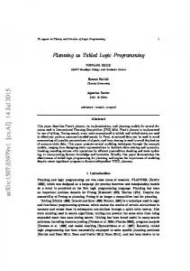
Figure 1 represents a possible state of the system during evaluation of the query :- p(X). against the program of Listing 1. Each tree is represented by a triangle inclosing a derivation tree. Edges between trees represent the dependence relation between consumer nodes and trees. In the remainder of the paper, we will abstract away the details of derivation trees, and concentrate on the trees in the system and the dependence relation among them, depicted in the form of edges. :- table p/1, q/1, r/1. p(X) :- q(X). q(X) :- r(X), s(X). r(a). r(X) :- r(Y), e(Y,X). s(d).
e(a,b). e(a,c). e(b,d). e(c,d).
Listing 1: Reachability
In fact, the dependence relation defines a multi-graph, where nodes are the trees in the system, and there is an edge for each consumer node, connecting the consuming tree to its supplier. We call this graph the Demand Graph, since it denotes a relation of demand and supply between tables. A demand graph is a weak approximation of the notion of Relevance defined in [11]. Definition 1 (Demand Graph) Given a snapshot of an SLG system, a Demand Graph DG (N, E, QN ) is a directed multi-graph where N is a set of nodes, each representing a tree in the SLG system, and E is the set of edges, representing the dependencies between trees. QN is the node representing the tree for the query being evaluated. This multi-graph expands as evaluation progresses and new trees and consumer nodes are created. In fact, in the absence of pruning operators, the graph only grows monotonically, until evaluation of the query is completed. Pruning introduces a non-monotonic component to the evaluation when undemanded trees are deleted. The desired semantics of once(P) states that P should succeed at most once. In other words, as soon as the first successful derivation for P is found, the associated consumer node should be marked such that the goal once(P) does not succeed again. If P contains variables, only one possible binding for each variable is returned. Assuming that P is a tabled predicate, applying the once operator on P essentially amounts to removing an edge from the demand graph of the system when P succeeds. Clearly, this removal may affect the connectivity of the graph, rendering some trees unreachable from the query tree. This state is captured by the concept of Demand on trees. Definition 2 (Demand on Trees) Given a demand graph DG (N, E, QN ), a node T1 is said to be demanded if there is a path in DG , from the query node QN to T1 . Similarly, if no such path exists, we say that T1 is undemanded.
Approximate Pruning in Tabled Logic Programming
73
For performance reasons, undemanded trees should not be scheduled for further evaluation, since there is no indication that other answers for them will be needed to evaluate the current query. Therefore, our algorithm eagerly detects undemanded trees when pruning occurs, and removes them from the set of active trees. Listing 2 shows pseudo-Prolog code for a demand-based once operator. We assume that nodes are created in a stack-like structure, so that get next node ref returns a reference to the next node to be created. A metacall starts evaluation of the subgoal P, creating a new node, which is referred to by R. After the meta-call returns, remove demand disconnects the consumer node referred to by R from the tree that supplies it. A reference to the query table is then obtained, and reachability from the query is computed. undemand trees removes all trees in the system that are not demanded from the scheduling set. once(P) :get_next_node_ref(R), call(P), remove_demand(R), query(Q), reachable(Q,Reach), undemand_trees(Reach).
undemand_trees(G) :table(T), ( not member(G,T) -> undemand_table(T) ; true ), fail. undemand_trees(_).
Listing 2: once implementation in Prolog
While it represents our desired semantics, an actual implementation of the algorithm in Listing 2 would present a few drawbacks. First, an expensive traversal of the demanded trees has to be performed each time pruning takes place. Also, a resumption mechanism is necessary, in order to re-impose demand on previously undemanded trees for which new consumers are created. Another point to notice is that it may be advantageous, from the point of view of memory management, to actually remove undemanded trees. In that case, if new calls to undemanded trees are created, these trees will have to be recomputed. On the other hand, if trees are never collected, memory usage may be problematic. We next define a safe approximation of a demand-based once operator, which attempts to delete trees when demand on them is released.
3
Approximate Pruning
We have argued, in the previous section, that implementing a pruning operation based on exact demand is hard, requiring a full reachability analysis over the evaluation graph. In this section we present an approximation of this operation aimed at preserving our desired semantics, while decreasing the implementation costs of pruning. In the following, we describe the intuitions behind our approximation, before presenting the pruning algorithm.
74
L.F. Castro and D.S. Warren
One issue related to pruning in Tabled Prolog systems is whether undemanded trees should be frozen, or completely deleted. Freezing trees allows for possible future calls to benefit from results already computed, and restart evaluation from that point on, if necessary. On the other hand, if these trees are never called again, deleting them is a more memory-efficient solution. The problem constitutes a tradeoff between evaluation time, which is minimized if trees are frozen, and memory usage, minimized when trees are deleted. The pruning operator presented here deletes trees whenever possible. When undemanded trees are deleted, recomputation may become an issue, possibly altering termination characteristics of programs. Even so, we believe there are many applications where keeping undemanded trees may turn out to consume excessive amounts of resources and adversely affect system performance. Another advantage of this approach is its simplicity. Supporting resumption of trees, besides requiring extra bookkeeping, impacts the scheduling mechanism in a non-trivial way. On the other hand, it may improve long-running computations significantly, when trees are reused, and thus recomputations avoided. A full demand-based pruning operation, as presented in the previous section, is able to select individual trees which become undemanded when a given edge is removed due to pruning. The algorithm we describe next uses an approximation to decide which trees to delete. The application of a pruning operation induces a scope. Intuitively, the scope consists of all those trees that have been created during the evaluation of the goal being pruned. The notion of scope captures all those trees which could potentially be deleted from the system as a result of this application of pruning. The fact that a table is in the scope of a pruning operation does not directly mean that it can be deleted, since it can still be demanded. Instead of selecting which trees continue to be demanded, and which do not, our approximation decides whether to delete in the level of a scope. When all trees in a scope are undemanded, then they are all deleted. Otherwise, all trees in the scope are maintained in the system. However, instead of freezing these trees, they are maintained as active, and new (possibly unnecessary) answers for these trees may be computed. While this may cause superfluous work to be done, the semantics is guaranteed by removing the connection between the specific subgoal being pruned and the table that supplies answers to it. In order to support this approximate pruning algorithm based on this notion of scope, we augment our evaluation model with timestamps that impose an ordering in events. Based on this extended model, the notion of scope is defined in terms of reachability over generator edges. Finally, the approximate pruning algorithm is presented and discussed. 3.1
Timestamped Forest of Trees
First we augment the concept of demand graph by introducing timestamps on its edges and trees. We assume a global counter of events is available, which is incremented each time a new edge is created. When an edge is created, it is tagged with the current value of the event counter. Also, trees are timestamped
Approximate Pruning in Tabled Logic Programming
75
with the value of the event counter at the time they are created. When no pruning takes place, each tree has the same timestamp as its oldest incoming edge. In fact, this edge has a special significance, and is called the Generator edge for that tree. Definition 3 (Generator edge) An edge is said to be the Generator edge of a tree Ti if its destination is Ti , and its timestamp coincides with that of Ti . We denote the timestamp of an edge e (tree t) as timestamp(e) (timestamp(t)). The source (destination) of an edge is defined in terms of the timestamp of the tree it points from (to). Definition 4 (Edge properties) Given an edge e, from tree Ts to tree Td , we define: source(e) = timestamp(Ts ) dest(e) = timestamp(Td ) Figure 2 shows the timestamps in the system depicted in Figure 1. Notice that the query tree has always a timestamp of 0. The main characteristic of approximate 2 1 pruning is that trees are only considered for 3 removal when their corresponding generator 1 2 0 edges are also removed. Removal of a nongenerator edge never causes a tree to be removed. Therefore, in order to decide which Fig. 2. Timestamps trees can be removed, we have to consider only those trees which are reachable via generator edges. The scope of a given application of once on a subgoal is, intuitively, the set of trees that may potentially be undemanded after the generator edge for the subgoal is removed. The scope is defined in terms of reachability over generator edges. We first define the Generator-Restricted Demand Graph as a restriction on the edges of a demand graph, such that only generator edges are included. Definition 5 (Generator-Restricted Demand Graph) Given a demand multi-graph DG (N, E, QN ), we define its induced generator-restricted demand G (N, E � , QN ), where E � is defined by E � = {e ∈ graph as the graph DG E | e timestamp(e) = dest(e)}. Generator-reachability is defined as reachability over the generator-restricted graph entailed by a given demand graph. Definition 6 (Generator-reachability) Given a demand graph DG (N, E, QN ), and an edge e ∈ E, we define Generator-reachability as the set of edges reachable from e in the Generator-restricted graph induced by DG . G reachG (e, DG (N, E, QN )) = {e� ∈ E | e� ∈ reach(e, DG )}
76
L.F. Castro and D.S. Warren
Finally, we define the scope of a pruning operation as the set of trees that are Generator-reachable from the edge being removed. Definition 7 (Scope) Given a demand graph DG (N, E, QN ) and an edge e ∈ E that is the direct subject of a once operation, we define the scope of the once operation as scope(e, DG ) = {e� ∈ reachG (e, DG )} Our algorithm is based on the principle that a pruning operation can only remove trees which appear in its scope. But the fact that a given tree t appears in a scope does not imply that it is not demanded. It may happen that there are other edges, in the demand graph, connecting nodes outside the scope to t, thus creating an alternate path from the query tree to t, which does not use the edge being removed. This alternative source of demand is called external demand. For example, consider the situation if Figure 3, where edge number 2 is being pruned. The scope, in this case, consists of trees 5 with timestamps 2, 3 and 4. But edge num4 3 2 1 ber 6 imposes an external demand on tree 4, so that this tree cannot be deleted. In this 1 2 3 4 0 case, approximate pruning removes edge 2, 6 but does not delete any trees, since there is external demand on the scope. Fig. 3. External Demand In order to detect whether a given scope has external demand, we need to inspect all edges coming into trees in the scope. If the source of any of these edges is a tree that is not in this scope, then there is external demand. Otherwise, the scope is undemanded. Definition 8 (External demand on a scope) Given a demand graph DG (N, E, QN ) and an edge e ∈ E that is the direct subject of a once operation, we define that the scope of this pruning operation is externally demanded as: / scope(e, DG )∧ external demand(e, DG (N, E, QN )) ⇐⇒ ∃e� ∈ E | source(e� ) ∈ dest(e� ) ∈ scope(e, DG ) 3.2
Approximate Pruning Algorithm
The algorithm for approximate pruning implementing the once operator is presented in Listing 3. It performs a meta-call on the subgoal being pruned, and releases demand on it after the meta-call succeeds. The algorithm is presented in a high-level Prolog form, and assumes the existence of the following builtin predicates, which form an interface for inspecting and manipulating the internally represented current demand graph. edge(Source,Dest,Timestamp). A set of facts that describe the edges of the demand graph;
Approximate Pruning in Tabled Logic Programming
77
timestamp(Timestamp). A builtin predicate that returns the current value of the timestamp counter; delete edge(Timestamp). Removes the edge given by Timestamp from the graph; delete tree(Timestamp). Removes the tree with timestamp Timestamp, and all edges outgoing from it.
once(SubGoal) :timestamp(Timestamp), call(SubGoal), delete_edge(Timestamp), ( generator(Timestamp) -> ( demanded_scope(Timestamp) -> true ; delete_scope(Timestamp) ) ; true ).
:- table gen_reach/2. gen_reach(Timestamp,Tree) :edge(Timestamp, Tree, Tree). gen_reach(Timestamp,Tree) :gen_reach(Timestamp,Tree1), edge(Tree1,Tree,Tree). delete_scope(Timestamp) :gen_reach(Timestamp,Tree), delete_tree(Tree), fail. delete_scope(_).
generator(Timestamp) :edge(_,Timestamp,Timestamp). demanded_scope(Timestamp) :edge(Source, Dest, Time), Time > Timestamp, not gen_reach(Source), gen_reach(Dest).
Listing 3: Pseudo-code for optimized version of once
The predicate once receives as argument a subgoal to be resolved. It starts by recording the current timestamp, which is the timestamp of the next edge to be created. The subgoal is called using Prolog’s meta-call builtin. Upon return of the meta-call, the edge corresponding to the subgoal is deleted, thus enforcing the desired semantics. Further optimization is performed by deleting the tables created during computation of the subgoal, whenever possible. The general algorithm presented in Section 2 performs reachability from the query tree in order to select, individually, which trees are undemanded and can be deleted. In this optimized algorithm, tree removal is decided in terms of the scope of the once operation. That is, if there is external demand on any tree in the scope, then no trees are removed; otherwise, all trees in the scope are deleted. This is performed by first checking whether the edge of the subgoal is a generator edge. In that case, demanded scope checks whether any tree in the scope of the subgoal has external demand. If so, nothing is done, otherwise delete scope
78
L.F. Castro and D.S. Warren
removes all trees in the scope from the system. Both demanded scope and delete scope are defined in terms of gen reach, which implements generatorreachability.
4
Implementation
We present an implementation of approximate pruning in the XSB Prolog[13] system. XSB is based on the SLG-WAM[8] abstract machine, a specialization of the original WAM[16]. We first provide a basic description of how XSB implements the SLG-WAM architecture, followed by a presentation of how the demand graph model is represented in the implementation.
4.1
SLG-WAM Architecture
Data areas in XSB are organized into four main stacks. The Heap maintains longlived structures and variables. The Local stack maintains the environments for clause-local variables, much like activation records in imperative languages. The Control and Trail stacks store information required to perform backtracking. Non-deterministic search in Prolog is implemented by backtracking. Each time a choice is encountered during execution, a choice-point is laid down in the Control stack. This stack works as a last-in-first-out source of alternatives. That is, when backtracking is necessary, the topmost choice-point in the Control stack is used. When a choicepoint is exhausted it can be discarded, and then its predecessor is taken as the next source of alternatives. SLG evaluation may require that a computation be suspended and other alternatives be executed, before it may be resumed. Suspended computations are represented by portions of the stacks in the system. It is left to the implementation to decide how these stack sections are to be maintained. Typically, these are either protected and kept in the stacks, as in the original formulation of the SLG-WAM[12], or copied to an outside area, as in CHAT [3]. In the remainder of this paper we assume a shared stack management as in the original SLG-WAM. Notice that, in order to recreate the context of a suspended computation, the system may need to redo bindings undone by backtracking while this computation was suspended. Thus, the Trail is augmented to keep the values that conditional variables are bound to [15], so that the engine can run the trail not just backwards, but also forwards, rebinding variables needed to reconstruct an earlier context. The central data-structure for table management is the Subgoal Frame. Each subgoal frame contains information about a variant call encountered during evaluation. Subgoal frames maintain references to the associated generator choicepoint for the call and for the answers already generated. Also, each subgoal frame maintains a list of all consumer choicepoints which consume from its associated table.
Approximate Pruning in Tabled Logic Programming
4.2
79
Mapping the Demand Graph onto XSB
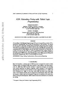
Table management and scheduling are essentially controlled by two datastructures in XSB. Subgoal frames centralize status information about trees in the system, and maintain references to all answers already found for the tree. Choicepoints represent internal nodes, and are classified into three main kinds. Prolog choicepoints are used to maintain unexplored choices in non-tabled predicate definitions. A generator choicepoint is created when the first call to a tabled predicate is encountered, and consumer choicepoints are laid down for calls to already-seen subgoals. Subgoal Frame p(X) Control Stack
Program :- table all. p(X) :- q(X),r(X),s(X). q(a). q(b). r(X) :- q(X). s(X) :- r(X),q(X). Query |-? q(X).
p(X) q(X) r(X)
Generator
Subgoal Frame q(X)
Generator Generator
q(X) Consumer s(X) r(X)
Generator
Subgoal Frame
Consumer
r(X)
q(X) Consumer
Subgoal Frame s(X)
Fig. 4. XSB structures and their relationship
As noted in Section 2, we are interested in those tree nodes 2 which generate dependencies be1 tween trees. In XSB, these are rep5 3 resented by the consumer and gen1 2 4 0 erator choicepoints. Generator choi6 cepoints have a dual role in XSB. p(X) q(X) r(X) s(X) Besides indicating that results from a given table Td are demanded from Fig. 5. Dependency Graph the callee table Ts , they also serve the purpose of performing clause resolution to generate answers for Td . Figure 4 shows an example of these structures during evaluation of a query, and their relationship. The corresponding dependency graph is shown in Figure 5. Generator choicepoints are linked to their corresponding subgoal frames, 4
80
L.F. Castro and D.S. Warren
and vice-versa. All consumers of a given table are chained together, and this chain is anchored in the subgoal frame of the table. This chain is called the consumer chain of the table. Summarizing, edges are represented by the choicepoints in the stack. Generator edges correspond to generator choicepoints, which are distinguished in the system. Trees are mapped to Subgoal frames, and their auxiliary structures, which are not presented here. We now examine how the operations necessary to implement our algorithm can be efficiently realized, and describe the changes to the standard SLG-WAM data structures necessary to support these operations. edge. The edge relation connects consuming trees to their suppliers. This relation is realized by consumer and generator choicepoints, and the timestamps for these edges are implicitly represented by the memory addresses of these choicepoints. Choicepoints already maintain references to the tables they are supplying, as shown in Figure 4 by the dashed arrows. Tables are connected to the consumers it supplies (dotted arrows). In order to provide fast access to the tree a given consumer is consuming from, we have augmented the SLG-WAM structure by creating a new chain that effectively transforms dotted arrows in Figure 4 into double arrows. delete edge. This function is responsible for ensuring that no more answers will be returned to a given choicepoint representing a tabled call. If the choicepoint is a consumer choicepoint, we simply delete it by removing it from the chain of choicepoints considered for scheduling. Generator choicepoints, as observed earlier, are responsible both for returning answers to a tabled call via its forward continuation, and for generating answers to a table, through its backwards continuation. When delete edge is applied to a generator choicepoint, it modifies its forward continuation to a failure, so that no answers will be returned to the tabled call, even though it remains able to generate answers to the table. delete tree. Given the timestamp of a table, which in SLG-WAM is represented by the address of its generator choicepoint, delete tree deletes its data structures and execution context. The Subgoal frame and all answers already computed for the table are deleted, as well as its generator choicepoint, and all consumers that supply this table. A precondition for delete edge is that no demand exists on the table it is applied to, so nothing is done with respect to consumers of this table. If there are consumers, they should be deleted when the tables they are supplying are deleted. gen reach. This predicate is used both to traverse all tables in the scope of the operation (as in demanded scope) and also as a simple check, as in demanded. gen reach is realized in the implementation by performing a reachability analysis in the beginning of the algorithm, marking all choicepoints which are reachable, and thus in the scope of pruning. This provides for an easy, constant-time check for whether a given choicepoint is in the scope. Traversal of choicepoints in the scope is performed, when necessary, by a linear scan of the top of the choicepoint stack, skipping those choicepoints not marked.
Approximate Pruning in Tabled Logic Programming
81
demanded scope. This predicate essentially collects all edges younger than the timestamp at entry of once, whose source is not in its scope. The key to implement this function is to realize that, since timestamps are implicitly represented by the address of choicepoints, a simple traversal of the top of the Control stack (back to the point where once started evaluation), selecting unmarked choicepoints, obtains all such edges. If any of these choicepoints consumes from a table in the scope of once, it means that the scope has external demand, and the predicate succeeds. This information is obtained by following the links from consumers to tables they supply (dashed lines in Figure 4.)
5
Experimental Results
Time (ms)
In this section, we present some quantitative data that suggests that approximate pruning, with table deletion, can significantly impact execution times of programs. In order to illustrate these 100 possible gains, we benchmark a No Pruning Pruning version of the classical Stalemate game depicted in Listing 4 10 in the form of the predicate win. Given a directed graph, this 1 game states that a node is a winner if there is an edge connect0.1 ing this node to a non-winner node. Nodes which have no possi0.01 10 15 20 25 30 35 ble moves are, by default, winner Depth of binary tree nodes. The goal is to determine if a given node is a winner node. Fig. 6. Performance comparison for the staleIt is important, in general, that mate game the win predicate be tabled, so that the evaluation terminates in the presence of cycles in the input graph. :- table win/0. win(X) :move(X,Y), tnot(win(Y)).
test(Depth) :create_bin_tree(Depth), cputime(T1), win(0), cputime(T2), Time is T2 - T1, write(time(win(Depth),Time)).
Listing 4: The Stalemate win/not-win game
It is clear that it is uninteresting to collect alternative proofs for the winning status of a given node. This can be easily obtained by ensuring that negation builtins like XSB’s tnot fail early when the first counter-proof is found. Cur-
82
L.F. Castro and D.S. Warren
rently, tnot does not perform pruning when it fails, so unnecessary computation is performed. We have adapted the tnot operator to take advantage of approximate pruning, and compared execution times using the test predicate of Listing 4. The test dynamically creates full binary trees with variable depth. Figure 6 shows results obtained for tests run both with and without the modified tnot builtin. It is clear that, even though pruning does not change the exponential nature of this problem, it significantly lowers the slope of the curve1 . Besides time, memory performance is important for this benchmark. In fact, we were unable to run the non-pruning version of the benchmark for trees of depth larger than 23 on a machine with 2Gb of memory. Another important point when introducing new functionality is to measure the impact the added machinery imposes when the functionality is not being used. We have benchmarked a set of non-pruning benchmarks on XSB with and without support for our pruning operator. The maximum overhead observed was about 3%.
6
Summary
The backward chaining evaluation model of Prolog computes only those subgoals that are needed in order to resolve a given query. Pruning allows for a finer control of determinism, which can be used to further extend this concept of performing only demanded computations. It can be used by the Prolog engine itself, in order to improve its evaluation strategy, and also by the programmer, so that she can annotate programs with control information. Tabled Prolog builds on the concept of demand-driven evaluation by allowing each relevant goal to be evaluated only once. But there are no satisfactory pruning operators in Tabled Prolog, since it is hard to decide which tables are demanded in the presence of suspension and resumption of subgoals. We have presented an abstraction of SLG evaluation where the SLG forest of trees is represented by a directed graph, and demand is defined in terms of reachability from a query node. This allowed us to define a demand-based once pruning operator. Full demand-based pruning is costly, so we presented sound approximate pruning in the form of a safe once operator. Approximate pruning uses a notion of the scope of the once operation as the basic unit for which demand is determined and implemented. This allows for an efficient pruning mechanism, which has been implemented in the XSB system. One question when performing pruning on tabled systems is whether undemanded tables should be deleted, or whether they should be kept in a scratch area, so that future calls could use their results, and re-impose demand on them. Approximate pruning takes the approach of deleting undemanded tables, given that their scope is currently undemanded. This has the advantage of early memory reclamation, but may have adverse effects on the termination characteristics 1
Notice that the y axis of the graph is plotted in a logarithmic scale.
Approximate Pruning in Tabled Logic Programming
83
of a program. We intend to study the alternative of maintaining undemanded trees, and supporting the re-imposition of demand on them. We believe each approach will prove effective in different situations.
References 1. K. A. M. Ali. A method for implementing cut in parallel execution of Prolog. In ICSLP’87. 2. W. Chen and D. S. Warren. Tabled Evaluation with Delaying for General Logic Programs. Journal of the ACM, 43(1):20–74, January 1996. 3. B. Demoen and K. Sagonas. CHAT: the Copy-Hybrid Approach to Tabling. In PADL’99, 1999. 4. H.-F. Guo and G. Gupta. A simple scheme for implementing tabled logic programming systems based on dynamic reordering of alternatives. In ICLP’01, pages 181–196, 2001. 5. H.-F. Guo and G. Gupta. Cuts in tabled logic programming. In B. Demoen, editor, CICLOPS’02, 2002. 6. G. Gupta and V. Santos Costa. Cuts and side-effects in and-or parallel prolog. Journal of Logic Programming, 27(1):45–71, 1996. 7. R. O’Keefe. The Craft of Prolog. MIT, 1990. 8. K. Sagonas and T. Swift. An abstract machine for tabled execution of fixed-order stratified logic programs. TOPLAS, 20(3):586–635, May 1998. 9. T. Swift. A new formulation of tabled resolution with delay. In Recent Advances in Artificial Intelligence. 10. T. Swift. Efficient Evaluation of Normal Logic Programs. PhD thesis, SUNY at Stony Brook, 1994. 11. T. Swift. A new formulation of tabled resolution with delay. In EPIA’99, 1999. 12. T. Swift and D. S. Warren. An abstract machine for SLG resolution: definite programs. In SLP’94, pages 633–654, 1994. 13. The XSB Programmer’s Manual: version 2.5, vols. 1 and 2, 2002. http://xsb.sourceforge.net/. 14. D. S. Warren. Programming in tabled prolog – DRAFT. Available from http://www.cs.stonybrook.edu/˜warren. 15. D. S. Warren. Efficient Prolog memory management for flexible control. In ILPS’84, pages 198–202, 1984. 16. D.H.D. Warren. An abstract Prolog instruction set. Technical Report 309, SRI, 1983.