a new tabled logic programming-based IP matching algorithm that can check .... Section 5 presents a design flow to illustrate where an IP matching tool fits and ...
Tabled Logic Programming-based IP Matching Tool using Forced Simulation
P. S. Roop
A. Sowmya
S. Ramesh
Haifeng Guo
Department of ECE
School of CSE
Department of CSE
Department of CS
University of Auckland University of New South Wales
Indian Institute of Technology
University of Nebraska at Omaha
Auckland - 1
Bombay 400 076
Omaha, NE 68182-0500
Sydney, 2052
1
Abstract Automatic IP (Intellectual Property) matching is a key to reuse of IP cores. This paper presents a new tabled logic programming-based IP matching algorithm that can check whether a given programmable IP can be adapted to match a given specification. When such adaptation is possible, the algorithm also generates a device driver (an interface) to adapt the IP. Though simulation, refinement and bisimulation based algorithms exist, they cannot be used to check the adaptability of an IP, which is the essence of reuse. The IP matching algorithm is based on a formal verification technique called forced simulation. A forced simulation based matching algorithm is implemented using a tabled logic programming environment, which provides distinct advantages for encoding such an algorithm. The tool has been used to match several specifications to programmable IPs, achieving on an average 12 times speedup and 64 % reduction in code size in comparison to previously published algorithms.
2
List of Figures 1
Abstract behaviour of Intel 8255 . . . . . . . . . . . . . . . . . . . . . . . . . . . .
7
2
Intel 8255 in mode 2 . . . . . . . . . . . . . . . . . . . . . . . . . . . . . . . . . .
8
3
The port of a lathe controller . . . . . . . . . . . . . . . . . . . . . . . . . . . . . .
9
4
An Interface Process . . . . . . . . . . . . . . . . . . . . . . . . . . . . . . . . . .
10
5
������
for the lathe controller port
. . . . . . . . . . . . . . . . . . . . . . . . . . .
12
6
Example of Justification Subtrees . . . . . . . . . . . . . . . . . . . . . . . . . . . .
19
7
Justification evidence for (a) matching action (b) forcing action . . . . . . . . . . . .
20
8
An IP Matching Process . . . . . . . . . . . . . . . . . . . . . . . . . . . . . . . .
3
23
1 Introduction 1.1 Motivation Design reuse has been the focus of recent research [8, 12] mainly driven by the increasing complexities of modern systems. Other major factors influencing this revolution are immense competition from vendors and consequently less time to market, the need for more open (generic) solutions of the Internet era, and most importantly the need for developing solutions that can be easily verified, often referred to as design for verifiability [3]. The advantages of design reuse are improved productivity, better performance and, more significantly, better quality products. In a recent survey on digital design reuse [8] several key factors for successful reuse of Intellectual Property (IP) cores have been identified. These include, among others, the need for synthesis techniques to support the reuse of predesigned IP blocks. The authors also identify a need for enabling reuse of a set of prevalidated IPs from a library. These features are not appropriately addressed in current synthesis tools. To automatically reuse IPs during synthesis, a subset of IPs is normally indexed from a database. Subsequent to indexing, matching is essential to identify the exact IP (a device
�
) that is functionally
equivalent to the design function ( ). Martin et al. [2001] have proposed a fuzzy logic based scoring and aggregation technique for indexing IPs from a distributed database that may possibly match a given
. After indexing, precise functionality matching is not proposed as part of this work and the
authors suggest simulation as a means for precise IP matching. Simulation can be a tedious and time consuming activity. In addition, exhaustive simulation may not guarantee that the selected IP is the desired one. This problem is even more severe with programmable or parameterisable IPs which may not exactly match device driver (an interface) to match
but can be programmed via a
. This paper proposes an algorithmic technique suitable for
�
fast logic programming-based implementation, for automatically deciding whether a given . The algorithm, when successful, automatically generates an interface
that can adapt
�
matches to match
. The basis of this algorithm is a formal verification technique called forced simulation [16] and hence is guaranteed to produce correct matches. This paper recasts forced simulation into the logic 4
programming framework for the following reasons: 1. Ease of implementation: the resulting code is extremely compact and readable. In contrast to about 1200 lines of Java code spanning 5 classes to compute forced simulation using partitionrefinement based approach [16], logic programming based encoding could be done in just 82 lines within the XSB tabled logic programming framework [17]. 2. Efficiency: the complexity of the logic programming based algorithm is less by a factor of
�� � ,
the size of the function specification. As a result the proposed approach achieves an average speed up of about 12 compared to the earlier implementation. 3. Interface generation as a side effect: XSB justifier was used to obtain an interface without a second pass over the constructed forced simulation relation. 4. Reasons for Failure: When the matching fails, the justifier can be used to discover the reasons for failure. Justification takes no more time than the original query evaluation. This additional feature is expensive to build into other implementations.
1.2 Related Work The task of IP matching is similar to simulation/refinement based verification in the sense that both need to establish whether a given IP (an implementation) meets all requirements of a specification. Several simulation/refinement techniques [1, 9] have been proposed in literature. During IP matching, however, a generic implementation often needs to be matched to a given specification. This is the essence of reuse. None of the existing simulation techniques can be used to adapt a generic implementation for a given specification. Forced simulation overcomes these limitations and has been reported in [16]. Forced simulation is a bisimulation variant and hence standard partition-refinement based bisimulation algorithms [4] may be modified for computing forced simulation [16]. This paper demonstrates the advantages of a tabled logic programming system such as XSB to implement a formal IP matching tool. XSB has already been used for building efficient model checkers and bisimulation checkers
5
[14]. Features of XSB such as tabling and constraint propagation can be exploited to build an efficient matching tool, with the additional facility of explaining failed matches whenever they occur. This paper is organised as follows: section 2 presents the formal framework for IP matching using forced simulation. The model and most definitions are identical to those presented in [16] and are reproduced for completeness. In addition, Definition 5, which recasts forced simulation to better fit the logic programming framework, is new but equivalent to the definition in [16]. Section 3 shows how the matching algorithm can be encoded in the XSB logic programming environment. This section also shows how the XSB justifier is used to automatically generate the interface after successful matching and also to explain failed matches. Section 4 presents some results of using the matching tool-kit developed in XSB and compares this to a conventional partition-refinement based implementation in Java. Section 5 presents a design flow to illustrate where an IP matching tool fits and section 6 is devoted to concluding remarks.
2 Forced Simulation: Formal Framework for Matching This section presents the formal framework of forced simulation as the basis of the matching algorithm. Because of the advantages of encoding the rules for computing the forced simulation relation as a logic program, the rules are redefined in an equivalent form to facilitate such an encoding. Hence, the theory of forced simulation as presented here is equivalent though different from [16]. At the outset, an example of a programmable port (Intel 8255) is presented to illustrate the idea. This illustrates how this IP may be programmed to be used as a port for a lathe controller.
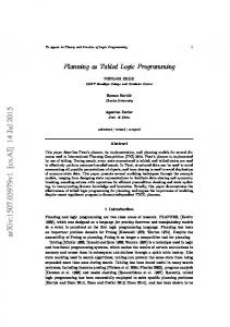
2.1 Reusing a general purpose port, Intel 8255 Intel 8255 [7] is a general purpose 8-bit parallel port. It can be used to interface I/O devices to a CPU. It has three 8-bit ports called PORT-A, PORT-B, and PORT-C, of which PORT-A and PORT-B are I/O ports, whereas PORT-C can be used as both an I/O port and control lines, depending on the mode of operation. Intel 8255 may be programmed to be in one of the following modes (Figure 1 shows the abstract
6
D: in−mode0
dev−init 0
1
2
mode−0
in−mode1 in−mode2
3
mode−1
4 mode−2
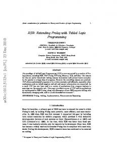
Figure 1: Abstract behaviour of Intel 8255 behaviour of the three modes and Figure 2 is the detailed behaviour in mode 2, which is the mode of interest to this example): 1. mode 0 (basic input-output mode): CPU may read contents of a port or write some data to it. 2. mode 1 (strobed input-output mode): This is mainly for reading or writing from a port using handshake protocol. 3. mode 2 (bidirectional bus): This mode is like mode 1 except that it can be used for bidirectional data transfer, while mode 1 is unidirectional. Consider the specification of a lathe controller, where Figure 3 provides an abstract description of a typical port used in such a controller. The function of this port is to read instructions written in a tape reader and then transfer these to the CPU in a handshaking fashion. The CPU interprets these instructions and writes appropriate lathe instructions to the port, which are read by the lathe to perform the appropriate lathe action. Figure 3 gives the abstract description of each transition of the handshaking sequence as comments.
7
mode2 STB=0
INTE1=1 4
28
STB=1 31
30
29
32
INTR=1 33
IBF=1
INTE2=1
DB=[PORT−A] 35
34 RD=0
36 IBF=0
INTR=0 37 WR=0 38 PORT−A=[DB] 39 WR=1 40 OBF=0 41
INTR=1
ACK=0 42 OBF=1 43 ACK=1 44
Figure 2: Intel 8255 in mode 2 2.1.1 Let
Reuse via Interface be the lathe controller port as shown in Figure 3 and let to match
and 2. In order for adapt
�
�
�
be Intel 8255 as shown in Figure 1
, a device driver (an interface, ) is needed which can dynamically
in the following ways:
�
1. When
is in state 0,
must provide the device initialisation command dev-init followed by
�
required mode word in-mode2 to bring forcing. After
�
reaches state 4,
control signals of
�
not present in
to state 4. Such actions of the interface are known as
must continue to force INTE1=1, INTE2=1, which are extra . Forcing is not just required from the initial state but may
be applied in any other state when required (such as say forcing of IBF=0 when
�
is in state
35). In the interface, forcing signals are enclosed in [ ] to clearly distinguish them from other signals. 2. When
����
�
reaches state 29 and in
with transition
is still in state 0, the interface must enable matching of transition
��� � �
in
�
. Such actions of the interface are known as matching.
8
F: arc2
arc1 0
1
arc3 2
3
arc1: STB=0 /*tape reader has sent data to port */
arc5
arc4
5
4
arc6
6 arc2: IBF=1 /*port sends acknowledgement to tape reader*/
arc7 7
arc3: INTR=1 /*port interrupts the CPU to transfer tape data*/
arc8 arc4: RD=0 /*CPU wants to read port to get tape data*/ 8 arc5: DB=[PORT−A] /*contents of port are placed on data bus*/
arc9 9 arc13
arc10
arc6: INTR=0 /*reading of data is finished; port withdraws interrupt request*/ arc7: WR=0 /*CPU wants to now transfer instructions to lathe*/
10 arc11
arc8: PORT−A=[DB] /*CPU writes instruction to Lathe*/ arc9: WR=1 /*write complete*/
11
arc10: OBF=0 /*signal lathe to read instruction */
arc12 arc11: ACK=0 /*acknowledgement from Lathe*/ 12
arc12: OBF=1 /*ack back to lathe from port −− two way handshaking*/ arc13: INTR=1/*interrupt CPU to signal that one cycle of data transfer is over
Figure 3: The port of a lathe controller While matching, disabling may also be required when state, not present in
�
has extra transitions from the matching
(not required in this example).
The interface must perform such forcing and matching steps until the desired behaviour is realised. Such an interface is shown in Figure 4. This example raises the following additional questions: 1. Given arbitrary pairs of
and
�
, how to decide whether an interface exists or not?
2. Given an interface for known pair of in
and
�
, how to ensure that
�
implements all behaviours
? In other words, when is the interface correct?
To address these issues, a formalisation of the above problem is provided in the next section.
9
0, 0 [dev−init] 0,1 [in−mode2] 0, 4 [INTE1=1] [INTE2=1]
0, 28
0, 29 STB=0 1, 30 IBF=1
INTR=1 2, 31 [STB=1] 2, 32
3, 33
INTR=1
RD=0
12, 44
4, 34
[ ACK=1 ]
DB=[PORT−A] WR=0 5, 35
5, 36
6, 37
PORT−A=[DB] 7, 38
ACK=0 9, 40
8, 39 WR=1
[IBF=0]
INTR=0
10,41 OBF=0
11, 42
12, 43
OBF=1
Figure 4: An Interface Process
2.2 Formalisation In the previous section, the reuse of Intel 8255 was illustrated via an interface process that adapts the IP for reuse. Hence, given a pair ( , of
and
�
�
), the main idea is to build an interface such that the composition
exhibits the same behaviour as
. First
,
�
and
are formalised by modelling them as
labelled transition systems [11] which are standard models of reactive processes. Definition 1 A process is described by a labelled transition system (LTS) which is a tuple of the form
����������� � ��
, where:
�
is a finite set of states,
��� ������� � events or signals and
� ��
�
is a unique start state,
�
�
��������� � ��� � �
�
is a finite set of
is the transition relation.
In this paper, it is assumed that all processes are deterministic. Let LTSs �� and
�
������� � � ����� �
stand for the function and device processes respectively.
Definition 2 An interface process, , is a process whose set of events is
10
��� �"! #%$'& #( )�+*
.
�
The new set of signals of the form
!# $
are the special signals that force the transitions labelled # in
the device. Any interface has normal transitions (called external moves) labelled by forced moves which are labelled by a forced move where the signal
#
in addition to
! # $ . For example, in Figure 4 the transition from the start state is
������� �� ��
is forced.
2.3 The IP Matching Problem Before the IP matching problem can be defined, the interaction between For this, a new parallel composition operator in
with a corresponding transition in
In addition, the
���
�
���
�
as above,
��������� ��� ��� ��� � ����� ��� ����������� ��� � �
transition relation
�
������
������� � � �
must be clarified.
that is forced to give an unobservable � move in
resulting in an observable external move in
�
�
was proposed in [16], which combines a forced move
operator combines an external move in
Definition 3 Given
and
�����
. The
���
������
with an identical external move in
.
�
operator is defined as follows:
is defined to be a process described by the LTS
�
where �������� � � �
�
� �
�
� �
and
� ������� ��� � �"! ��� *
and the
������� � � � is defined by the following rules: �����
1. Forced Move: �
� makes an unobservable � move, when forces a transition in
�
.
#%$'+�& (*, ) #%$.-0/1#02 +3( , 0# 245 # $ /1# 2%68+�7 , 5 # $�- /1# 42 -�6 2. External Move: �
�����
� makes an observable move, with both
�
and
simultaneously re-
sponding to the same external signal.
#%$ +�( , %# $.-0/1#02 +3( , 0# 245 # $ /1# 2%6 � + (, 5 # $�- /1# 42 -�6 Note that the
���
operator is quite different from synchronous parallel ( & & ) operator of CCS [11].
Firstly, unlike synchronous parallel operator, the new operator disallows autonomous moves. Secondly, forced move is different from synchronous parallel with global hiding, as forcing essentially leads to state based hiding. For the lathe controller port example in the previous section,
�����
is
shown in Figure 5. For
�
to match ,
�����
must be behaviourally equivalent to . This is checked by using Milner’s
weak bisimulation [11] (denoted as 9 and also known as observational equivalence). Intuitively, two 11
0
τ
1
τ
2
τ
3
τ 4 STB=05
6
INTR=1
τ 7
DB=[PORT−A]
8
IBF=1
9
10
INTR=0 τ
12
11
RD=0
WR=0 13 PORT−A=[DB] 14 WR=1 15
INTR=1
OBF=0 16 ACK=0 17 OBF=1 18 τ 19
Figure 5:
������
for the lathe controller port
processes are weakly bisimilar if their behaviour cannot be distinguished by an external observer. Note that, for the lathe controller port example of the previous section, the behaviour of is observationally equivalent to internal � steps of
������
������
in Figure 5 (the only difference between
�����
and
in Figure 3 are some
which are anyway not observable).
The IP matching problem is now formalised as follows: Definition 4 A device
�����
such that �
� 9
�
can implement a function
(
�
matches
) if there exists an interface
where 9 is Milner’s weak bisimulation [11].
In the following section, a relation between the states of
and
�
, called forced simulation, is
defined. It is then established that the existence of such a forced simulation relation is a necessary and sufficient condition for successful IP matching.
2.4 Condition for Matching: Forced Simulation For an IP
�
to match a specification
, an appropriate
must be constructed such that �
To achieve this, a new simulation relation, called forced simulation between the states of
12
������
� 9
and
�
. is
defined. It is then shown that
�
and
. In this case,
A pair
and
some states in
�
�
exists if and only if a forced simulation relation
can be constructed from
algorithmically, as presented in the next section.
are said to be forced similar if there exists a relation
� �
�
�
�
Two states
��
are related over R if either they are directly related or related via a forcing
and
��
are directly related if for every transition
�� � � ��
��
in
�
and further
��
�
and �
��
�
�
� � �� ��� �
��
�
�
and
��
are related via a forcing sequence
is reachable from
���
via path
�
(see Definition 4). Whenever
�� � �� ��
��
in
, there is a matching
are also related over R. In this case, �
Definition 4).
such that
to
and
sequence .
Two states
relating states of
.
Two states
transition
holds between
and further
��
and
��
�
�
�
� � (see
� � ����� �
if there exists a successor state and
��
��
�
��
in
�
are directly related. In this case,
are related, then the states of the tuple ( �
� ����� )
(in Figure 2) from section 2.1. State 0 in
(de-
match. Consider the example of
�
(in Figure 3) and
� � ) is not directly related to state 0 in � (denoted � � � ) as they do not have matching transitions. However, � � � is directly related to � �� �� as they do have matching transitions and their successors � �� � and � ��� � are also directly related. As � �� �� is reachable from ��� � by a path triggered by events � � � � � �� � ����� ��� � � � � � ���� � � ���� � � , � � � and � � � are related by a forcing sequence. It is easy to establish that � � � is related by forcing sequences to � ��� , ����� and � �� �� . By continuing in this noted �
manner, a forced simulation relation may be constructed between the states of
and
�
, is defined
below. Definition 5 Given LTSs
and
�
�
�� � �
�
is a forced simulation relation (in short,
� ) provided: � � � ����� ��� � �! ���#" � � �� � ��� �%$ �'&(�� )�*)���+,�-+�. ���0/ ���2� 1 �����3 � �� � �4�� � ) � � � where � � ����� ��� � ���� ���#" � �5� �4�� �6& ���7� �4���3 ���� �4�� ). Forced simulation, as originally proposed [16], required a forcing sequence � to be associated with �
an f simulation relation where �
��
, a relation
���
is a shorthand for �
� � �� ��� �
�
a device state ��� that will force it to be similar to a function state � . Intuitively, the role of the forcing 13
sequence is to indicate the sequence of inputs required to guide
��
�� , reachable ��
to a successor state,
�� has similar behaviour as � � . However, for logic programming encoding, carrying
from ��� such that �
� Definition 6 � ��� ���
around explicit ’s is difficult and unnecessary. Definition 4 overcomes this difficulty.
�
�
, whenever there exists an f simulation relation between them.
2.5 Results The following two theorems state that forced simulation is a necessary and sufficient condition for IP
�
matching (where
and
Theorem 1 Given
� ��� ���
are represented as LTSs).
�
there exists
such that
9
����� �
�.
Theorem 2 If there exists a well-formed and deterministic interface
� ��� ���
�
such that
����� 9
then
.
The proof of both these theorems are constructive and appear in [16]. Theorem 1 and 2 form the formal basis (necessary and sufficient condition) for IP matching. As is obvious, a key to IP matching is the identification of an appropriate interface to adapt the IP. This is achieved by identifying a forced simulation relation first, and then constructing an interface from it. The next section demonstrates how and why logic programming is employed for these tasks.
3 Logic Programming Based IP Matching Forced simulation is an extension of a standard verification technique called bisimulation [11]. Normally, bisimulation algorithms are implemented using bottom-up partition refinement [4]. A similar bottom-up algorithm for forced simulation has been already developed in [16]. This algorithm starts by constructing a global relation set of all reachable states in tively. The size of this set
�
which is initialised to
���
�
�
� �
�
�
�
� where
�
�
�
� is the
�� � # � ��� denote the number of states of and � respec� � ����(� �� � � since � � � � is � � � � � . � � � � is is � � � �
. Let
required for computing the forcing sequences. After computing
14
the algorithm refines it by using
a partition-refinement-like algorithm until a greatest fixed point is reached. The complexity of this implementation has been shown to be of transitions in
�
� � � � � �� � � �
� where
�
denotes the maximum number
.
Unlike bottom-up algorithms that construct the maximal relation and then refine it until the greatest fixed point is reached, logic programming systems such as XSB operate in a top-down manner
� ����� ) are forced similar. This local decision making results in a reduction in complexity by a factor of � � . XSB and explore only states that are required to prove (or disprove) that a given pair of ( �
based encoding is very small, simple and hence readable. This is because, unlike bottom-up implementations which require code to be written for creation, manipulation and traversal of graph data structures, XSB uses a set of logical facts to represent the graphs corresponding to
and
�
, and
forced simulation is encoded as a set of rules. Additionally, the XSB justifier can be used to generate the interface, and to generate evidence for the matching, taking no more time than the original query evaluation.
3.1 Encoding of forced simulation in XSB Rather than encoding the forced simulation relation directly, it is more convenient to encode the dual of forced simulation as a tabled logic program within XSB. This is because XSB is a least fixed point engine whereas forced simulation computation is based on a greatest fixed point (the greatest forced simulation relation between
and
�
is computed when it exists).
The rules for a pair of states to be not-forced-similar are directly encoded as XSB clauses. Input datasets
and
�
are encoded as a set of facts representing the adjacency matrix of the corresponding
LTSs. For example, consider the LTS of the lathe controller port function (Figure 3). The corresponding encoding of the above in XSB as a set of simple Prolog facts is given below: trans(f(0), ’STB=0’, f(1)). trans(f(1), ’IBF=1’, f(2)). trans(f(2), ’INTR=1’, f(3)). trans(f(3), ’RD=0’, f(4)).
15
trans(f(4), ’DB=[PORT-A]’, f(5)). trans(f(5), ’INTR=0’, f(6)). trans(f(6), ’WR=0’, f(7)). trans(f(7), ’PORT-A=[DB]’, f(8)). trans(f(8), ’WR=1’, f(9)). trans(f(9), ’OBF=0’, f(10)). trans(f(10), ’ACK=0’, f(11)). trans(f(11), ’OBF=1’, f(12)). trans(f(12), ’INTR=1’, f(0)). In the above, trans encodes a given transition where the first and the last parameters indicate the source and destination states and the second parameter indicates the input that triggers this transition.
�
For example, the first fact indicates that there is a transition from state the to the state triggered by the input
� ��
�
.
In the following, we provide the formal definition and the corresponding encoding in XSB. Suppose
�
�
is a forced simulation relation, then
, the dual of
, is defined as :
� ����� � � � �'��� ��� � � � ) ��+,�-+�. ���� / ��� � 1 � �� 3 � � �� � �� ��� where, � � �'����� & � 5 � � � �4�� � ����� � ���� 3 �4�� ����
�����
�
��� �
� � ����� � is not forced similar (denoted by � � ��� ) when � � is not directly forced similar to � � (denoted � � � ��� ) and all reachable states ���� from ��� are also not directly forced similar to � � . A given pair � � � ����� � is not directly forced similar whenever � � has a transition that cannot be matched to any transition from This definition is the equivalent of Definition 4 and encodes the fact that a pair �
���
. Also, note that since
�
is a deterministic LTS, the above may be rewritten by replacing the
& giving: & � �5� � ���� �6& ���7� � 4� ���3 ���� �� �� .
quantification to a
�
� � �����
is the least model of the above formula, and is encoded as a logic program in XSB as follows: :- table nfsim/2. nfsim(SF, SD) :-
16
nfsim_e(SF, SD), findall((SD,SD1), (reach(SD,SD1), SD\=SD1), SL), all_nfsim_e(SF, SL). all_nfsim_e(_, []). all_nfsim_e(SF, [(SD, SD1)|R]) :nfsim_e(SF, SD1), all_nfsim_e(SF, R). nfsim_e(SF, SD) :trans(SF, A, _), \+ trans(SD, A, _). nfsim_e(SF, SD) :trans(SF, A, SF1), trans(SD, A, SD1), nfsim(SF1, SD1).
In the above, nfsim/2, a tabled predicate, denotes the dual relation
, and nfsim e/2 the relation
�� .
findall(X, Goal, List) collects all the instances of X to List such that Goal is provable. If Goal is not provable, List will be an empty list []. The predicate all nfsim e/2 is used to verify the relation
� between a state in � �
with each state from the given list of states in
���
where
\+ stands for negation. The tabled predicate reach/2 is used to determine reachable successors and is encoded as: :- table reach/2. reach(S, S1) :- trans(S, _A, S1). reach(S, S1) :- trans(S, _A, S2), reach(S2, S1).
�
��
An LTS
����� � ����� �
, then trans( � ,
#
is encoded as a set of facts in a logic program
, ) is in
. Note that since
�%�
�
as well as
such that whenever
# �
are from a finite
set, they can be represented in a logic program by ground terms. Thus, given the coding of forced simulation, and two LTSs states �
��
and
���
, the query, to check whether
� ��� ��� 17
�
and
�
with their respective start
is satisfied or not, is nfsim( �
��,
��� �
).
3.2 Query and Its Justification Query evaluation of a goal with respect to a logic program establishes the truth or falsehood of the goal. Given two LTSs
��� �
and
�
with their respective start states
) is performed to check whether
��� ���
�
���
and
���
, the query nfsim( �
��,
is satisfied or not. When such a similarity relation
exists, an interface is then generated to specify forcing and matching actions in detail. In the case of failure to construct such a relation, some critical unmatched states should be provided as evidence of the failure. The XSB system provides an efficient justifier [5] for giving evidence, in terms of proof, for the truth value of the result generated by query evaluation of a tabled logic program. For example, if a query is evaluated to true, the justifier will present the details of a successful computation path, suppressing any unsuccessful paths traversed. Similarly, when a query is evaluated to false, it will show the false literal, leading to falsehood of the query, in each of its computation paths. Justification succinctly conveys to the user only those parts of the proof search which are relevant to the proof/disproof of the goal. The naturalness of using a tabled LP system for justification is that the answer memo tables created represent the lemmas that were tried and possibly proved during query evaluation. By using these lemmas stored in the tables, the justifier presents only relevant parts of the derivation to the user. The justification result is in the form of a tree structure [5], constructed based on a collection of partial structures. The partial structures, e.g., as shown in Figure 6, show the proof dependencies, which are actually determined by the coding rules defined in section 3.1. Figure 6(a) and (b) correspond to the coding of all nfsim e/2 and nfsim/2 respectively, where findall/3 and trans/3 are defined as the fact nodes in the structure since the evidence for those predicates are not interesting. Each node is associated with a truth value to indicate whether it is satisfiable or not. In Figure 6(b), nfsim(F,D) is true, which means that there is no forced simulation relation between and
�
, and its children in the tree explain why this is so.
18
nfsim(F,D) TRUE
all_nfsim_e(F,[(D,D1)|R]) TRUE nfsim_e(F,D1) TRUE all_nfsim_e(SF,R) TRUE
Justification of nsfim_e/2
nfsim_e(F,D) TRUE
all_nfsim_e(F,L) TRUE
findall((D,D1),(reach(D, D1),D\=D1),L) TRUE Justification of nsfim_e/2
Justification of all_nfsim_e/2
(a)
Justification of all_nfsim_e/2
(b) Figure 6: Example of Justification Subtrees
3.3 Interface Generation An interface generator was implemented within XSB by defining a few rewriting rules from the justification results at the logic programming level. The generated interface is essentially a high-level justification for an LTS-based device a forced simulation relation
��� � �
� �
to realise the specified LTS-based function
if there exists
, or, otherwise, a partial simulation that points out the state
from which no further simulation can be made. An interface process, as in Figure 4, can be described by a collection of matching actions and forcing actions. The rewriting rules are thus defined from certain justification structures to actions. They determine the meaning of a justification tree by determining the meanings of its substructures and combining them into a complete interface process. Two types of moves, matching action and forced action, must be explicitly shown in a generated interface process. Matching actions can be defined as follows:
�
�
�����
�
,
�
�� ���#" � �� � ���#" �
� � � 4� �� �6& ����� � �� ���3 �4�� 4� �� ,
corresponding to the structure in Figure 7(a), where the truth value of a node being false means that
19
its negated literal is true. For example, (SF1, SD1)
� � � 333� �
false. Then, all the transition labels
���
means that nfsim(SF1, SD1) is
in Figure 7(a) are matching actions. On the
� can be defined as: � � ����� � � �� ���#" �'&(�� � )�/ ���21 �4���3 � �� �'���� � ,
whose structure is shown in Figure 7(b), where the reachable path from
�
�
other hand, a sequence of forced actions
� �
,
to
� �
� is the sequence
of forced actions . The corresponding interface is shown in Figure 4. Note: SL = [D1 | SL1] SL i = [D i+1 | SLi+1 ] (1