On Combining Linear-Based Strategies for Tabled Evaluation of Logic ...

Under consideration for publication in Theory and Practice of Logic Programming

1

arXiv:1107.5030v2 [cs.LO] 26 Jul 2011

On Combining Linear-Based Strategies for Tabled Evaluation of Logic Programs MIGUEL AREIAS and RICARDO ROCHA CRACS & INESC-Porto LA, Faculty of Sciences, University of Porto Rua do Campo Alegre, 1021/1055, 4169-007 Porto, Portugal (e-mail: {miguel-areias,ricroc}@dcc.fc.up.pt) submitted 1 January 2003; revised 1 January 2003; accepted 1 January 2003

Abstract Tabled evaluation is a recognized and powerful technique that overcomes some limitations of traditional Prolog systems in dealing with recursion and redundant sub-computations. We can distinguish two main categories of tabling mechanisms: suspension-based tabling and linear tabling. While suspension-based mechanisms are considered to obtain better results in general, they have more memory space requirements and are more complex and harder to implement than linear tabling mechanisms. Arguably, the SLDT and DRA strategies are the two most successful extensions to standard linear tabled evaluation. In this work, we propose a new strategy, named DRS, and we present a framework, on top of the Yap system, that supports the combination of all these three strategies. Our implementation shares the underlying execution environment and most of the data structures used to implement tabling in Yap. We thus argue that all these common features allows us to make a first and fair comparison between these different linear tabling strategies and, therefore, better understand the advantages and weaknesses of each, when used solely or combined with the others. KEYWORDS: Linear Tabling, Integration, Implementation.

1 Introduction The operational semantics of Prolog is given by SLD resolution (Lloyd 1987), an evaluation strategy particularly simple that matches current stack based machines particularly well, but that suffers from fundamental limitations, such as in dealing with recursion and redundant sub-computations. Tabled evaluation (Tamaki and Sato 1986; Chen and Warren 1996) is a recognized and powerful technique that can considerably reduce the search space, avoid looping and have better termination properties than SLD resolution. Tabling consists of storing intermediate solutions for subgoals so that they can be reused when a repeated subgoal appears during the resolution process. Implementations of tabling are currently available in systems like XSB Prolog (Sagonas and Swift 1998), Yap Prolog (Rocha et al. 2000), B-Prolog (Zhou et al. 2000), ALSProlog (Guo and Gupta 2001), Mercury (Somogyi and Sagonas 2006) and Ciao

2

Miguel Areias and Ricardo Rocha

Prolog (de Guzm´ an et al. 2009). In these implementations, we can distinguish two main categories of tabling mechanisms: suspension-based tabling and linear tabling. Suspension-based tabling mechanisms need to preserve the computation state of suspended tabled subgoals in order to ensure that all solutions are correctly computed. A tabled evaluation can be seen as a sequence of sub-computations that suspend and later resume. Linear tabling mechanisms use iterative computations of tabled subgoals to compute fix-points and for that they maintain a single execution tree without requiring suspension and resumption of sub-computations. While suspension-based mechanisms are considered to obtain better results in general, they have more memory space requirements and are more complex and harder to implement than linear tabling mechanisms. Arguably, the SLDT (Zhou et al. 2000) and DRA (Guo and Gupta 2001; Areias and Rocha 2010) strategies are the two most successful extensions to standard linear tabling evaluation. As these strategies optimize different aspects of the evaluation, they are, in principle, orthogonal to each other and thus it should be possible to combine both in the same system. However, to the best of our knowledge, no single Prolog system supports both strategies simultaneously and thus, understanding the advantages and weaknesses of each cannot be fully dissociated from the base Prolog system on top of which they are implemented. In this work, we propose a new strategy, named Dynamic Reordering of Solutions (DRS), and we present a framework, on top of the Yap Prolog system, that integrates and supports the combination of the SLDT, DRA and DRS strategies. Our implementation shares the underlying execution environment and most of the data structures used to implement tabling in Yap (Rocha et al. 2000). In particular, we took advantage of Yap’s efficient table space data structures based on tries (Ramakrishnan et al. 1999), which we used with minimal modifications. We thus argue that all these common support features allows us to make a first and fair comparison between these different linear tabling strategies and, therefore, better understand the advantages and weaknesses of each, when used solely or combined with the others. The remainder of the paper is organized as follows. First, we briefly introduce the basics of tabling and describe the execution model for standard linear tabled evaluation. Next, we present the SLDT, DRA and DRS strategies and discuss how they can be used to optimize different aspects of the evaluation. We then provide some implementation details regarding the integration of the three strategies on top of the Yap engine. Finally, we present some experimental results and we end by outlining some conclusions.

2 Standard Linear Tabled Evaluation Tabling works by storing intermediate solutions for tabled subgoals so that they can be reused when a repeated call appears1 . In a nutshell, first calls to tabled subgoals

1

A subgoal call repeats a previous call if they are the same up to variable renaming.

On Combining Linear-Based Strategies for Tabled Evaluation

3

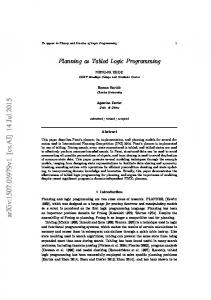
are considered generators and are evaluated as usual, using SLD resolution, but their solutions are stored in a global data space, called the table space. Repeated calls to tabled subgoals are considered consumers and are not re-evaluated against the program clauses because they can potentially lead to infinite loops, instead they are resolved by consuming the solutions already stored for the corresponding generator. During this process, as further new solutions are found, we need to ensure that they will be consumed by all the consumers, as otherwise we may miss parts of the computation and not fully explore the search space. A generator call C thus keeps trying its matching clauses until a fix-point is reached. If no new solutions are found during one cycle of trying the matching clauses, then we have reached a fix-point and we can say that C is completely evaluated. However, if a number of subgoal calls is mutually dependent, thus forming a Strongly Connected Component (SCC), then completion is more complex and we can only complete the calls in a SCC together (Sagonas and Swift 1998). SCCs are usually represented by the leader call, i.e., the generator call which does not depend on older generators. A leader call defines the next completion point, i.e., if no new solutions are found during one cycle of trying the matching clauses for the leader call, then we have reached a fix-point and we can say that all subgoal calls in the SCC are completely evaluated. We next illustrate in Fig. 1 the standard execution model for linear tabling. At the top, the figure shows the program code (the left box) and the final state of the table space (the right box). The program defines two tabled predicates, a/1 and b/1, each defined by two clauses (clauses c1 to c4). The bottom sub-figure shows the evaluation sequence for the query goal a(X). Generator calls are depicted by black oval boxes and consumer calls by white oval boxes. Call

:- table a/1, b/1. a(X):- b(X). a(2). b(X):- a(X). b(1).

1: a(X)

(c1) (c2) (c3) (c4)

2: b(X)

c2 7: X=2

2: b(X)

3: a(X)

c2

9: b(X)

15: X=1 (repeated)

6: X=1

c3

c1

X=1 X=2 complete X=1 X=2 complete

8,18,28: fix-point check

1: a(X)

c1 2: b(X)

Solutions 6: 7: 28: 4: 12: 28:

17: X=2 (repeated)

19-27: ...

16: X=2 (repeated)

5: fix-point check

9: b(X)

c4

c3 10: a(X)

4: X=1

11: X=1 (repeated)

14: fix-point check

c4 13: X=1 (repeated)

12: X=2

Fig. 1. A standard linear tabled evaluation The evaluation starts by inserting a new entry in the table space representing

4


the generator call a(X) (step 1). Then, a(X) is resolved against its first matching clause, clause c1, calling b(X) in the continuation. As this is a first call to b(X), we insert a new entry in the table space representing b(X) and proceed as shown in the bottom left tree (step 2). Subgoal b(X) is also resolved against its first matching clause, clause c3, calling again a(X) in the continuation (step 3). Since a(X) is a repeated call, we try to consume solutions from the table space, but at this stage no solutions are available, so execution fails. We then try the second matching clause for b(X), clause c4, and a first solution for b(X), X=1, is found and added to the table space (step 4). We then follow a local scheduling strategy and execution fails (Freire et al. 1996). With local scheduling, new solutions are only returned to the calling environment when all program clauses were explored. The execution thus fails back to node 2 and we check for a fix-point (step 5), but b(X) is not a leader call because it has a dependency (consumer node 3) to an older call, a(X). Remember that we reach a fix-point when no new solutions are found during the last cycle of trying the matching clauses for the leader call. Next, as we are following a local scheduling strategy, the solution for b(X) should now be propagated to the context of the previous call. We thus propagate the solution X=1 to the context of the generator call for a(X), which originates a first solution for a(X), X=1 (step 6). Then, we try the second matching clause for a(X) and a second solution, X=2, is found and added to the table space (step 7). We then backtrack again to the generator call for a(X) and because we have already explored all matching clauses, we check for a fix-point (step 8). We have found new solutions for both a(X) and b(X), thus the current SCC is scheduled for re-evaluation. The evaluation then repeats the same sequence as in steps 2 and 3 (now steps 9 and 10), but at this time the consumer call for a(X) has solutions in the table. Solution X=1 is first forwarded to it, which originates a repeated solution for b(X) (step 11) and thus execution fails. Then, solution X=2 is also forward to it and a new solution for b(X) is found. In the continuation, we find another repeated solution for b(X) (step 13) and we fail a second time in the fix-point check for b(X) (step 14). Again, as we are following a local scheduling strategy, the solutions for b(X) are propagated to the context of the generator call for a(X), but only repeated solutions are found (steps 15 and 16). Clause c2 is then explored, but without any further developments (step 17). We then backtrack one more time to the generator call for a(X) and because we have found a new solution for b(X) during the last iteration, the current SCC is scheduled again for re-evaluation (step 18). The re-evaluation of the SCC does not find new solutions for both a(X) and b(X) (steps 19 to 27). Thus, when backtracking again to a(X) we have reached a fix-point and because a(X) is a leader call, we can declare the two subgoal calls to be completed (step 28). 3 Linear Tabling Strategies The standard linear tabling mechanism uses a naive approach to evaluate tabled logic programs. Every time a new solution is found during the last round of evaluation, the complete search space for the current SCC is scheduled for re-evaluation.


5

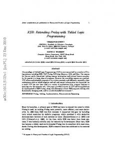
However, some branches of the SCC can be avoided, since it is possible to know beforehand that they will only lead to repeated computations, hence not finding any new solutions. Next, we will present three different strategies for optimizing the standard linear tabled evaluation. The common goal of these strategies is to minimize the number of branches to be explored, thus reducing the search space, and each strategy tries to focus on different aspects of the evaluation to achieve it. 3.1 Dynamic Reordering of Execution The first optimization, that we call Dynamic Reordering of Execution (DRE), is based on the original SLDT strategy, as proposed by Zhou et al. (Zhou et al. 2000). The key idea of the DRE strategy is to give priority to the program clauses instead of consuming answers, and to achieve that it lets repeated calls to tabled subgoals execute from the backtracking clause of the former call. A first call to a tabled subgoal is called a pioneer and repeated calls are called followers of the pioneer. When backtracking to a pioneer or a follower, we use the same strategy, first we explore the remaining clauses and only then we try to consume solutions. The fixpoint check operation is still only performed by pioneer calls. Figure 2 uses the same example from Fig. 1 to illustrate how DRE evaluation works. Call


1: a(X)

(c1) (c2) (c3) (c4)

1: a(X)

Solutions 4: 9: 19: 5: 6: 19:

2: b(X)


10,19: fix-point check

3: a(X)

c1

c2

2: b(X)

4: X=2 11-18: ...

8: X=2 (repeated)

9: X=1 2: b(X)

c3 3: a(X)

7: fix-point check

c4 6: X=1

5: X=2

Fig. 2. Using the DRE strategy to evaluate the program in Fig. 1 As for the standard strategy, the evaluation starts with first (pioneer) calls to a(X) (step 1) and b(X) (step 2), and then, in the continuation, a(X) is called repeatedly (step 3). But now with DRE evaluation, a(X) is considered a follower and thus we steal the backtracking clause of the former call at node 1, i.e., the second matching clause for a(X), clause c2. The evaluation then proceeds as for a generator call (right upper tree in Fig. 2), which means that new solutions can be generated for a(X). We thus try c2, and a first solution for a(X), X=2, is found and added to the table space (step 4). We then follow a local scheduling strategy and execution fails backtracking to the follower node. As both matching clauses for

6


a(X) were already taken, we try to consume solutions. The solution X=2 is then propagated to the context of b(X) which originates the solution X=2 (step 5). Next, in step 6 we find the second solution for b(X) and in step 7 we check for a fix-point, but b(X) is not a leader call because it has a dependency (follower node 3) to an older call, a(X). The solutions for b(X) are then propagated to the context of the pioneer call for a(X), which originates a second solution for a(X), X=1 (step 9). We then backtrack to the pioneer call for a(X) and because we have already explored the matching clause c2 in the follower node 3, we check for a fix-point. Since we have found new solutions during the last iteration, the current SCC is scheduled for re-evaluation (step 10). The re-evaluation of the SCC does not find any further solutions (steps 11 to 18), and thus the evaluation can be completed at step 19. 3.2 Dynamic Reordering of Alternatives The key idea of the Dynamic Reordering of Alternatives (DRA) strategy, as originally proposed by Guo and Gupta (Guo and Gupta 2001), is to memoize the clauses (or alternatives) leading to consumer calls, the looping alternatives, in such a way that when scheduling an SCC for re-evaluation, instead of trying the full set of matching clauses, we only try the looping alternatives. Initially, a generator call C explores the matching clauses as in standard linear tabled evaluation and, if a consumer call is found, the current clause for C is memoized as a looping alternative. After exploring all the matching clauses, C enters the looping state and from this point on, it only tries the looping alternatives until a fix-point is reached. Figure 3 uses again the same example from Fig. 1 to illustrate how DRA evaluation works. Call


1: a(X)

(c1) (c2) (c3) (c4)

2: b(X)

c2 7: X=2

Looping Alternatives


3: c1

3: c3


1: a(X)

c1 2: b(X)

Solutions 6: 7: 24: 4: 12: 24:

c1 9: b(X) 17-23: ...

14: X=1 15: X=2 (repeated) (repeated)

6: X=1

2: b(X)

c3 3: a(X)

5: fix-point check

9: b(X)

c4

13: fix-point check

c3 4: X=1

10: a(X)

11: X=1 (repeated)

12: X=2

Fig. 3. Using the DRA strategy to evaluate the program in Fig. 1 The evaluation sequence for the first SCC round (steps 2 to 7) is identical to the


7

standard evaluation of Fig. 1. The difference is that this round is also used to detect the alternatives leading to consumers calls. We only have one consumer call at node 3 for a(X). The clauses in evaluation up to the corresponding generator, call a(X) at node 1, are thus marked as looping alternatives and added to the respective table entries. This includes alternative c3 for b(X) and alternative c1 for a(X). As for the standard strategy, the SCC is then scheduled for two extra re-evaluation rounds (steps 9 to 15 and steps 17 to 23), but now only the looping alternatives are evaluated, which means that the clauses c2 and c4 are ignored. 3.3 Dynamic Reordering of Solutions The last optimization, that we named Dynamic Reordering of Solutions (DRS), is a new proposal that can be seen as a variant of the DRA strategy, but applied to the consumption of solutions. The key idea of the DRS strategy is to memoize the solutions leading to consumer calls, the looping solutions. When a non-leader generator call C consumes solutions to propagate them to the context of the previous call, if a consumer call is found, the current solution for C is memoized as a looping solution. Later, if C is scheduled for re-evaluation, instead of trying the full set of solutions, it only tries the looping solutions plus the new solutions found during the current round. In each round, the new solutions leading to consumer calls are added to the previous set of looping solutions. In Fig. 4, we use again the same example from Fig. 1 to illustrate how DRS evaluation works. Call

Solutions

Looping Solutions


1: a(X)

(c1) (c2) (c3) (c4)

2: b(X)

c2 7: X=2

9: b(X)

16: X=2 (repeated)

5: fix-point check

2: b(X)

3: a(X)

c2 18-24: ...

15: X=2 (repeated)

6: X=1

c3

c1



1: a(X)

c1 2: b(X)

6: 7: 25: 4: 12: 25:

9: b(X)

c4

c3 4: X=1

10: a(X)

11: X=1 (repeated)

14: fix-point check

c4 13: X=1 (repeated)

12: X=2

Fig. 4. Using the DRS strategy to evaluate the program in Fig. 1 In this example, we only have one non-leader generator call, b(X), which is called once for each evaluation round over the SCC (steps 2, 9 and 18 in Fig. 4). By following the evaluation, it is possible to verify that no solutions are marked as looping solutions, and thus, on each round, b(X) only consumes the new solutions

8


found during the round. This means that solution X=1 only is consumed on the first round (step 6), solution X=2 only is consumed on the second round (step 15) and no solution is consumed on the last round.

4 Implementation Details This section describes some implementation details regarding the integration of the three strategies on top of the Yap engine, with particular focus on the table space data structures and on the tabling operations. 4.1 Table Space To implement the table space, Yap uses tries which is considered a very efficient way to implement the table space (Ramakrishnan et al. 1999). Tries are trees in which common prefixes are represented only once. Tries provide complete discrimination for terms and permit look up and insertion to be done in a single pass. Figure 5 details the table space organization for the example used on the previous sections. As other tabling engines, Yap uses two Table Space levels of tries: one for table entry table entry for a/1 for b/1 the subgoal calls and other for the comVAR0 VAR0 puted solutions. A subgoal trie subgoal trie tabled predicate accesses the table space subgoal frame subgoal frame for a(VAR0) for b(VAR0) through a specific table entry data struc1 2 1 2 ture. Each different solution trie solution trie subgoal call is represented as a unique path in the subgoal Fig. 5. Table space organization trie and each different solution is represented as a unique path in the solution trie. A key data structure in this organization is the subgoal frame. Subgoal frames are used to store information about each tabled subgoal call, namely: the entry point to the solution trie; the state of the subgoal (ready, evaluating or complete); support to detect if the subgoal is a leader call; and support to detect if new solutions were found during the last round of evaluation. The DRE, DRA and DRS strategies extend the subgoal frame data structure with the following extra information: DRE: the pioneer call; and the backtracking clause of the former call. DRA: support to detect, store and load looping alternatives; and two new states, loop ready and loop evaluating, used to detect, respectively, generator and consumer calls in re-evaluating rounds. DRS: support to detect, store and load looping solutions.


9

As these extensions are specific to each strategy, as we will see next, they can be combined without major overheads. 4.2 Tabling Operations We next introduce the pseudo-code for the main tabling operations required to support the integration of the three strategies on top of Yap. We start with Fig. 6 showing the pseudo-code for the new solution operation. Initially, the operation simply inserts the given solution SOL in the solution trie structure for the given subgoal frame SF and, if the solution is new, it updates the SgFr new solutions subgoal frame field to TRUE. If DRS mode is enabled for the subgoal, it also marks the newest solution found during the current round. We then implement a local scheduling strategy and always fail at the end. new_solution(solution SOL, subgoal frame SF) { if (solution_check_insert(SOL,SF) == TRUE) { // new solution SgFr_new_solutions(SF) = TRUE if (DRS_mode(SF) && first_solution_in_current_round(SF) == NULL) first_solution_in_current_round(SF) = SOL } fail() // local scheduling }

Fig. 6. Pseudo-code for the new solution operation Figure 7 shows the pseudo-code for the tabled call operation. New calls to tabled subgoals are inserted into the table space by allocating the necessary data structures. This includes allocating and initializing a new subgoal frame to represent the given subgoal call (this is the case where the state of SF is ready). In such case, the tabled call operation then updates the state of SF to evaluating; stores a new generator node2 ; and proceeds by executing the current alternative. On the other hand, if the subgoal call is a repeated call, then the subgoal frame is already in the table space, and three different situations may occur. First, if the call is already evaluated (this is the case where the state of SF is complete), the operation consumes the available solutions by implementing the completed table optimization which executes compiled code directly from the solution trie structure associated with the completed call (Ramakrishnan et al. 1999). Second, if the call is a first call in a re-evaluating round (this is the case where the state of SF is loop ready), the operation updates the state of SF to loop evaluating; stores a new generator node; and proceeds by re-executing the first looping alternative or the first matching alternative, according to whether the DRA mode is enabled or disabled for the subgoal. Third, if the call is a consumer call (this is the case where the state of SF is evaluating or loop evaluating), the operation first marks the current branch as 2

Generator, consumer and follower nodes are implemented as WAM choice points extended with some extra fields.

10


tabled_call(subgoal call SC) { SF = subgoal_check_insert(SC) // SF is the subgoal frame for SC if (SgFr_state(SF) == ready) { // first round SgFr_state(SF) = evaluating store_generator_node() goto execute(current_alternative()) } else if (SgFr_state(SF) == loop_ready) { // re-evaluation round SgFr_state(SF) = loop_evaluating store_generator_node() if (DRA_mode(SF)) goto execute(first_looping_alternative()) else goto execute(first_alternative()) } else if (SgFr_state(SF) == evaluating or // first round SgFr_state(SF) == loop_evaluating) { // re-evaluation round mark_current_branch_as_a_non_leader_branch(SF) if (DRA_mode(SF) or DRS_mode(SF)) mark_current_branch_as_a_looping_branch(SF) if (DRE_mode(SF) && has_unexploited_alternatives(SF)) { store_follower_node() if (DRA_mode(SF) and SgFr_state(SF) == loop_evaluating) goto execute(next_looping_alternative()) else goto execute(next_alternative()) } else { store_consumer_node() goto consume_solutions(SF) } } else if (SgFr_state(SF) == complete) // already evaluated goto completed_table_optimization(SF) }

Fig. 7. Pseudo-code for the tabled call operation

a non-leader branch and, if in DRA or DRS mode, it also marks the current branch as a looping branch. Next, if DRE mode is enabled and there are unexploited alternatives (i.e., there is a backtracking clause for the former call), it stores a follower node and proceeds by re-executing the next looping alternative or the next matching alternative, according to whether the DRA mode is enabled or disabled for the subgoal. Otherwise, it stores a new consumer node and starts consuming the available solutions. To mark the current branch as a non-leader branch, we follow all intermediate generator calls in evaluation up to the generator call for frame SF and we mark them as non-leader calls (note that the call at hand defines a new dependency for the current SCC). To mark the current branch as a looping branch, we follow all intermediate generator calls in evaluation up to the generator call for frame SF and we mark the alternatives being evaluated or the solutions being consumed by each call, respectively, as looping alternatives or looping solutions. Finally, we discuss in more detail how completion is detected. Remember that after exploring the last matching clause for a tabled call, we execute the fix-point check operation. Figure 8 shows the pseudo-code for its implementation. The fix-point check operation starts by checking if the subgoal at hand is a leader call. If it is leader and has found new solutions during the current round, then the


11

fix-point_check(subgoal frame SF) { if (SgFr_is_leader(SF)){ if (SgFr_new_solutions(SF)) { // start a new round SgFr_new_solutions(SF) = FALSE for each (subgoal in current SCC) SgFr_state(subgoal) = loop_ready SgFr_state(SF) = loop_evaluating if (DRA_mode(SF)) goto execute(first_looping_alternative()) else goto execute(first_alternative()) } else { // complete subgoals in current SCC for each (subgoal in current SCC) SgFr_state(subgoal) = complete goto completed_table_optimization(SF) // local scheduling } else { // not a leader call if (SgFr_new_solutions(SF)) // propagate new solutions SgFr_new_solutions(current_leader(SF)) = TRUE SgFr_new_solutions(SF) = FALSE // reset new solutions // local scheduling if (DRS_mode(SF)) goto consume_looping_solutions_and_solutions_in_current_round(SF) else goto consume_solutions(SF) } }

Fig. 8. Pseudo-code for the fix-point check operation current SCC is scheduled for a re-evaluation. If it is leader but no new solutions were found during the current round, then we have reached a fix-point and thus, the subgoals in the current SCC are marked as completed and the evaluation proceeds with the completed table optimization. Otherwise, if the subgoal is not a leader call, then it propagates the new solutions information to the current leader of the SCC and starts consuming the available solutions. If DRS mode is enabled, it only consumes the looping solutions and the solutions found during the current round, otherwise it consumes all solutions.

5 Experimental Results To the best of our knowledge, Yap is now the first tabling engine that integrates and supports the combination of different linear tabling strategies. We have thus the conditions to better understand the advantages and weaknesses of each strategy when used solely or combined with the others. In what follows, we present initial experiments comparing linear tabled evaluation with and without support for the DRE, DRA and DRS strategies. The environment for our experiments was a PC with a 2.83 GHz Intel(R) Core(TM)2 Quad CPU and 4 GBytes of memory running the Linux kernel 2.6.32-27-generic-pae with Yap 6.0.7. To put the performance results in perspective, we used two right recursive definitions of the well-known path/2 predicate, that computes the transitive closure in a graph, combined with several different configurations of edge/2 facts. One path definition has the recursive clause first and the other has the recursive clause last.

12


path_first(X,Z) :- sld1, edge(X,Y), path_first(Y,Z), sld2. path_first(X,Z) :- sld3, edge(X,Z), sld4. path_last(X,Z) :- sld3, edge(X,Z), sld4. path_last(X,Z) :- sld1, edge(X,Y), path_last(Y,Z), sld2.

Regarding the edge facts, we used three configurations: a pyramid, a cycle and a grid configuration (Fig. 9 shows an example for each configuration). We experimented the pyramid and cycle configurations with depths 1000, 2000 and 3000 Pyramid Cycle Grid and the grid configuration with depths 20, (depth 3) (depth 3) (depth 3) 30 and 40. All experiments find all the solutions for the problem. We chose these Fig. 9. An example of edge configuraexperiments because the path/2 predicate tions implements a relatively easy to understand pattern of computation and its right recursive definition creates several interdependencies between tabled subgoals. Notice also that in the definitions above we included four extra SLD (non-tabled) predicates (the sld1/0, sld2/0, sld3/0 and sld4/0 predicates) in order to measure how the mixing with SLD computations can affect the base performance. First, in Table 1, we show the execution time, in milliseconds, for standard linear tabled evaluation with local scheduling and the ratios comparing standard linear tabling against DRE, DRA and DRS solely and combined strategies (All means DRE+DRA+DRS) for the two definitions of the path/2 predicate without including the four extra SLD computations. Ratios higher than 1.00 mean that the respective strategies have a positive impact on the execution time. The results obtained are the average of ten runs for each configuration. In addition to the results presented in Table 1, we also collected several statistics regarding important aspects of the evaluation (not fully presented here due to lack of space). In Table 2, we show some of these statistics for standard linear tabled evaluation and the ratios against the several strategies for the particular evaluation of the grid configuration with depth 40. The Alts column shows the number of alternatives explored during the evaluation, the Sols column shows the number of solutions consumed by generator nodes corresponding to non-leader subgoals, and the SLD columns show the number of times each extra SLD predicate is executed. Analyzing the general picture of Table 1, the results show that, for most of these experiments, DRE evaluation has no significant impact in the execution time. On the other hand, the results indicate that the DRA and DRS strategies are able to effectively reduce the execution time for most of the experiments, when compared with standard evaluation, and that by combining both strategies it is possible to obtain even better results. We next discuss in more detail each strategy. DRE: for most of these configurations, DRE has no significant impact. For the configurations with the recursive clause last and the configurations without loops (i.e., without inter-dependencies between subgoals), like the pyramid configura-


13

Table 1. Execution time, in milliseconds, for standard linear tabling with local scheduling and the respective ratios against the several strategies using the right recursive definition of the path problem (ratios in bold mean that the use of the respective strategies is better than not using some or all of them) Strategy

1000

Pyramid 2000 3000

1000

Cycle 2000

3000

20

Grid 30

40

Recursive Clause First Standard 664 2,669 DRE 1.02 1.01 DRA 1.55 1.51 DRS 1.01 1.00 DRE+DRA 1.52 1.51 DRE+DRS 1.01 1.01 DRA+DRS 1.54 1.52 All 1.56 1.53

6,040 1.02 1.51 1.01 1.50 1.00 1.51 1.50

377 1.00 1.22 1.21 1.24 1.22 1.56 1.55

1,522 1.01 1.23 1.23 1.23 1.23 1.57 1.57

3,400 1.01 1.21 1.22 1.20 1.22 1.52 1.52

386 1.02 1.14 1.23 1.15 1.22 1.42 1.38

2,714 1.00 1.09 1.27 1.10 1.23 1.42 1.39

10,689 1.00 1.10 1.31 1.06 1.23 1.43 1.37

Recursive Clause Last Standard 673 2,775 DRE 0.99 1.01 DRA 1.47 1.49 DRS 0.99 0.99 DRE+DRA 1.49 1.34 DRE+DRS 1.00 0.99 DRA+DRS 1.47 1.47 All 1.49 1.48

6,216 1.01 1.47 1.01 1.43 1.01 1.46 1.09

382 1.01 1.24 1.20 1.24 1.23 1.55 1.48

1,542 1.01 1.22 1.21 1.22 1.22 1.54 1.56

3,487 1.01 1.22 1.23 1.22 1.23 1.53 1.55

365 1.02 1.15 1.21 1.14 1.22 1.42 1.42

2,602 1.03 1.13 1.27 1.12 1.27 1.43 1.44

10,403 1.03 1.11 1.30 1.10 1.30 1.43 1.45

tions, it is not applicable and thus no followers nodes are ever stored. For the cycle configurations the number of followers is also very reduced, maximum 3 followers, and thus its impact is insignificant. For the grid configurations with the recursive clause first, the results obtained are the most interesting. For example, in Table 2 for the recursive clause first, DRE executes less alternatives (ratio 1.05) and consumes less solutions on non-leader generator nodes (ratio 1.04) than standard evaluation, but even so the impact on the execution time is minimal. DRA: the results for DRA evaluation show that the strategy of avoiding the exploration of non-looping alternatives in re-evaluation rounds is quite effective in general. The results also show that DRA is more effective for programs without loops (thus without looping alternatives), like the pyramid configurations, than for programs with larger SCCs, like the cycle and grid configurations. For the pyramid and grid configurations, the total number of alternatives explored by the other strategies is around 2 times the total number of alternatives explored with DRA. For the cycle configurations, this number is around 1.5 times the number with DRA evaluation. For example, in Table 2, we can observe that standard evaluation explores 1.91 times more alternatives (respectively 33,601 and 32,002

14


Table 2. Statistics for standard linear tabling and the respective ratios against the several strategies for the grid configuration with depth 40 (ratios in bold mean that the use of the respective strategies is better than not using some or all of them) Strategy

Alts

Sols

sld1/0

SLD Computations sld2/0 sld3/0

sld4/0

Recursive Clause First Standard 70,403 50,015,215 DRE 1.05 1.04 DRA 1.91 1.00 DRS 1.00 19.55 DRE+DRA 1.06 1.04 DRE+DRS 1.05 19.55 DRA+DRS 1.91 19.55 All 1.06 19.55

35,202 1.05 1.00 1.00 1.05 1.05 1.00 1.05

200,974,309 1.04 1.05 1.29 1.10 1.33 1.38 1.43

35,201 1.05 21.99 1.00 1.07 1.05 21.99 1.07

149,757 1.04 12.00 1.00 1.11 1.04 12.00 1.11

Recursive Clause Last Standard 67,204 48,080,300 DRE 1.00 1.00 DRA 1.91 1.00 DRS 1.00 18.79 DRE+DRA 1.91 1.00 DRE+DRS 1.00 18.79 DRA+DRS 1.91 18.79 All 1.91 18.79

48,602 1.00 1.00 1.00 1.00 1.00 1.00 1.00

352,277,129 1.00 1.05 1.29 1.05 1.29 1.38 1.38

48,602 1.00 20.99 1.00 20.99 1.00 20.99 20.99

205,920 1.00 11.50 1.00 11.50 1.00 11.50 11.50

more alternatives for the recursive clause first and last) than DRA evaluation for the grid configuration with depth 40. DRS: the results for DRS evaluation show that the strategy of avoiding the consumption of non-looping solutions in re-evaluation rounds is quite effective for programs that can benefit from it, like the cycle and grid configurations, and do not introduces relevant costs for programs that cannot benefit from it, like the pyramid configurations. Notice that the pyramid configurations only execute one re-evaluation round per SCC and that we only take advantage of DRS evaluation starting from the second re-evaluation round. For the cycle and grid configuration, DRS optimization is used several times because these configurations create a single huge SCC including all subgoal calls. For example, in Table 2, DRS consumes 47,456,815 (ratio 19.55) and 45,521,900 (ratio 18.79) less solutions than standard evaluation for the recursive clause first and last, respectively. Regarding the combination of the strategies, in general, our statistics show that the best of each world is always present in the combination. By analyzing the results in Table 1, we can conclude that, for these experiments, by combining the DRA and DRS strategies it is possible to reduce even further the execution time of the evaluation, and in most cases this reduction is higher than the sum of the reductions obtained with each strategy individually. In particular, Table 2 shows


15

the same number of solutions and alternatives for DRA+DRS that the respective DRS and DRA strategies obtain when used solely. This clearly shows the potential of our framework and suggests that the overhead associated with this combination is negligible. When DRE is present, the results are, in general, worse than the results obtained with the DRA/DRS strategies solely. In Table 2 we can observe that, for the DRE+DRA combination, the number of the alternatives explored is far more higher than the DRA used solely and that, for the DRE+DRS combination, the non consumed solutions for DRE used solely are included on the non consumed solutions of the DRS optimization. So, for this particular configurations, DRE is not fully orthogonal to DRA and DRS. Table 2 also shows the number of times each extra SLD predicate is executed for the grid configuration with depth 40. We can read these numbers as an estimation of the performance ratios that we will obtain if the execution time of the corresponding SLD predicate clearly overweights the execution time of the other tabled and nontabled computations. In particular, the sld2/0 predicate (placed at the end of the recursive clause) is the one that can potentially have a greater influence in the performance ratios as it clearly exceeds all the others in the number of executions. In general, these ratios show that by mixing tabled with non-tabled computations, our framework can achieve similar and, for some cases, even better results than the ones presented in Table 1. In particular, the ratios for the sld2/0 predicate (the one with greater influence) are very similar to the ratios in Table 1 and for DRA evaluation, the ratios for the sld3/0 and sld4/0 predicates are excellent (around 22 and 12, respectively), showing that intertwining SLD computations with linear tabling can affect positively the base performance.

6 Conclusions We presented a new strategy for linear tabled evaluation of logic programs, named DRS, and a framework that integrates and supports the combination of DRS with two other (DRE and DRA) linear tabling strategies. We discussed how these strategies can optimize different aspects of a tabled evaluation and we presented the relevant implementation details for their integration on top of the Yap system. Our experiments for DRS evaluation showed that the strategy of avoiding the consumption of non-looping solutions in re-evaluation rounds can be quite effective for programs that can benefit from it, with insignificant costs for the other programs. Preliminary results for the combined framework were also very promising. In particular, the combination of DRA with DRS showed the potential of our framework to reduce even further the execution time of a linear tabled evaluation. Further work will include adding new strategies/optimizations to our framework, such as the ones proposed in (Zhou et al. 2008), and exploring the impact of applying our strategies to more complex problems, seeking real-world experimental results, allowing us to improve and consolidate our current implementation.

16

Miguel Areias and Ricardo Rocha Acknowledgments

This work has been partially supported by the FCT research projects HORUS (PTDC/EIA-EIA/100897/2008) and LEAP (PTDC/EIA-CCO/112158/2009). References Areias, M. and Rocha, R. 2010. An Efficient Implementation of Linear Tabling Based on Dynamic Reordering of Alternatives. In International Symposium on Practical Aspects of Declarative Languages. Number 5937 in LNCS. Springer-Verlag, 279–293. Chen, W. and Warren, D. S. 1996. Tabled Evaluation with Delaying for General Logic Programs. Journal of the ACM 43, 1, 20–74. ´ n, P. C., Carro, M., and Hermenegildo, M. V. 2009. Towards a Complete de Guzma Scheme for Tabled Execution Based on Program Transformation. In International Symposium on Practical Aspects of Declarative Languages. Number 5418 in LNCS. SpringerVerlag, 224–238. Freire, J., Swift, T., and Warren, D. S. 1996. Beyond Depth-First: Improving Tabled Logic Programs through Alternative Scheduling Strategies. In International Symposium on Programming Language Implementation and Logic Programming. Number 1140 in LNCS. Springer-Verlag, 243–258. Guo, H.-F. and Gupta, G. 2001. A Simple Scheme for Implementing Tabled Logic Programming Systems Based on Dynamic Reordering of Alternatives. In International Conference on Logic Programming. Number 2237 in LNCS. Springer-Verlag, 181–196. Lloyd, J. W. 1987. Foundations of Logic Programming. Springer-Verlag. Ramakrishnan, I. V., Rao, P., Sagonas, K., Swift, T., and Warren, D. S. 1999. Efficient Access Mechanisms for Tabled Logic Programs. Journal of Logic Programming 38, 1, 31–54. Rocha, R., Silva, F., and Santos Costa, V. 2000. YapTab: A Tabling Engine Designed to Support Parallelism. In Conference on Tabulation in Parsing and Deduction. 77–87. Sagonas, K. and Swift, T. 1998. An Abstract Machine for Tabled Execution of FixedOrder Stratified Logic Programs. ACM Transactions on Programming Languages and Systems 20, 3, 586–634. Somogyi, Z. and Sagonas, K. 2006. Tabling in Mercury: Design and Implementation. In International Symposium on Practical Aspects of Declarative Languages. Number 3819 in LNCS. Springer-Verlag, 150–167. Tamaki, H. and Sato, T. 1986. OLDT Resolution with Tabulation. In International Conference on Logic Programming. Number 225 in LNCS. Springer-Verlag, 84–98. Zhou, N.-F., Sato, T., and Shen, Y.-D. 2008. Linear Tabling Strategies and Optimizations. Theory and Practice of Logic Programming 8, 1, 81–109. Zhou, N.-F., Shen, Y.-D., Yuan, L.-Y., and You, J.-H. 2000. Implementation of a Linear Tabling Mechanism. In Practical Aspects of Declarative Languages. Number 1753 in LNCS. Springer-Verlag, 109–123.