Retroactive Subsumption-Based Tabled Evaluation of Logic Programs

Retroactive Subsumption-Based Tabled Evaluation of Logic Programs Fl´ avio Cruz and Ricardo Rocha? CRACS & INESC-Porto LA, Faculty of Sciences, University of Porto Rua do Campo Alegre, 1021/1055, 4169-007 Porto, Portugal {flavioc,ricroc}@dcc.fc.up.pt

Abstract. Tabled evaluation is a recognized and powerful implementation technique that overcomes some limitations of traditional Prolog systems in dealing with recursion and redundant sub-computations. Tabling based systems use call similarity to determine if a tabled subgoal will produce their own answers or if it will consume from another subgoal. While call variance has been a very popular approach, call subsumption can yield superior time performance and space improvements as it allows greater reuse of answers. However, the call order of the subgoals can greatly affect the success and applicability of the call subsumption technique. In this work, we present an extension, named Retroactive Call Subsumption, that supports call subsumption by allowing full sharing of answers between subsumed/subsuming subgoals, independently on the order in which they are called. Our experiments using the YapTab tabling engine show considerable gains in evaluation time for some applications, at the expense of a very small overhead for the programs that cannot benefit from it. Keywords: Tabled Evaluation, Call Subsumption, Implementation.

1

Introduction

Tabling [1] is an implementation technique that solves some of the shortcomings of Prolog systems based on the traditional SLD resolution method. Tabled resolution methods can considerably reduce the search space, avoid looping and have better termination properties than SLD resolution based methods. The tabling technique is a refinement of SLD resolution that stems from one simple idea: save intermediate answers from past computations so that they can be reused when a similar call appears during the resolution process. In a nutshell, first calls to tabled subgoals are evaluated as usual, using SLD resolution, but their answers are stored in a global data space, called the table space. Similar calls to tabled subgoals are then resolved by consuming the answers already stored in the table entry for the corresponding similar subgoal, instead of being re-evaluated against the program clauses. Call similarity thus determines if a subgoal will ?

This work has been partially supported by the FCT research projects STAMPA (PTDC/EIA/67738/2006) and HORUS (PTDC/EIA-EIA/100897/2008).

produce their own answers or if it will consume from another subgoal. In general, we can distinguish two main approaches to determine similarity between tabled subgoals: variant-based tabling and subsumption-based tabling. In variant-based tabling, two subgoals are considered to be similar if they are the same by renaming the variables. For example, subgoals p(X, 1, Y ) and p(Y, 1, Z) are variants because both can be made identical to p(V AR0 , 1, V AR1 ) through variable renaming. In subsumption-based tabling, two subgoals are considered to be similar if one subgoal subsumes the other. A subgoal R is subsumed by a subgoal S (or a subgoal S subsumes a subgoal R) if R is more specific than S (or S is more general then R). For example, subgoal p(X, 1, 2) is subsumed by subgoal p(Y, 1, Z) because there is a substitution {Y = X, Z = 2} that makes p(X, 1, 2) an instance of p(Y, 1, Z). Notice that, if R is subsumed by S, S will contain in its table entry the full set of answers that also satisfy R and thus, R can reuse and consume answers directly from S. In general, subsumption-based tabling can yield superior time performance, as it allows greater reuse of answers, and better space usage, since the answer sets for the subsumed subgoals are not stored. However, the mechanisms to efficiently support subsumption-based tabling are more complex and hard to implement, which makes variant-based tabling more popular within the available tabling systems. To the best of our knowledge, until now, XSB Prolog was the unique system supporting subsumption-based tabling. The first implemented design was called Dynamic Threaded Sequential Automata (DTSA) [2], but was later replaced by an alternative table space organization called Time-Stamped Trie (TST) [3], that showed better space efficiency than DTSA. Despite the good results and performance gains obtained with the DTSA and TST designs, both approaches suffer from a major problem: the order in which subgoals are called during a particular evaluation can greatly affect the success and applicability of the call subsumption technique. For example, consider again the subgoals p(X, 1, 2) and p(Y, 1, Z). If p(X, 1, 2) is called after p(Y, 1, Z), then p(X, 1, 2) will be able to consume answers from p(Y, 1, Z) tables. Otherwise, if p(X, 1, 2) is called before, then no sharing will be possible, since answer reuse only happens when more general subgoals appear before specific ones. In this work, we present an extension to the original TST design, named Retroactive Call Subsumption (RCS), that supports call subsumption by allowing full sharing of answers between subsumed/subsuming subgoals, independently on the order in which they are called. The RCS proposal implements a strategy that allows retroactive sharing of answers among subgoals by means of selectively pruning and restarting the evaluation of subsumed subgoals. In order to support this, we introduce the following main extensions for subsumption-based tabling: (i) a new algorithm to efficiently traverse the table space searching for subsumed subgoals; (ii) a new table space organization, based on the ideas of the common global trie proposal [4], where answers are represented only once; and (iii) a new evaluation strategy to selectively prune and restart the evaluation of tabled nodes. We will focus our discussion on a concrete implementation, the YapTab system [5], but our proposals can be generalized and applied to other tabling

systems. Notice that, in order to do this work, first we have ported, from XSB Prolog to YapTab, the full code that implements the TST design1 . The remainder of the paper is organized as follows. First, we briefly introduce the main background concepts about tabled evaluation in YapTab. Next, we present the RCS proposal and discuss the main operational challenges involved in its design. We then describe how we have extended YapTab to provide engine support for it. Finally, we present some experimental results and conclusions.

2

Tabled Evaluation in YapTab

Tabling consists of storing intermediate answers for subgoals so that they can be reused when a similar subgoal appears. Whenever a tabled subgoal is first called, a new entry is allocated in the table space. Table entries are used to keep track of subgoal calls and to store their answers. Each time a tabled subgoal is called, we know if it is a repeated call by inspecting the table space searching for a similar call. Within this model, the nodes in the search space are classified as either: generator nodes, if they are being called for the first time; consumer nodes, if they are repeated calls; or interior nodes, if they are non-tabled subgoals. To support tabled evaluation, the YapTab design [5] extends the Warren’s Abstract Machine (WAM) [6] execution model with the following four operations: Tabled Subgoal Call: this operation searches the table space looking for a subgoal S similar to the current subgoal C being called. If such subgoal is found, C will be resolved using answer resolution and for that it allocates a consumer node and starts consuming the set of available answers from S. If not, C will be resolved using program clause resolution and for that it allocates a generator node, adds a new entry to the table space and initializes it with an empty set AC of answers. New Answer: this operation checks whether a newly found answer a for a generator node C is already in its table entry. If a is a repeated answer, the operation fails. Otherwise, a new answer set A0C = AC ∪ a is generated. Answer Resolution: this operation checks whether a consumer node C has new answers available for consumption. If no answers are available, C is suspended and execution proceeds using a specific strategy [7]. Consumers must suspend because new answers may still be found by the corresponding variant/subsuming call S. Otherwise, given C’s last consumed answer, we determine the unconsumed answer set UC ⊆ AS and consume the next one. Completion: this operation determines whether a subgoal S is completely evaluated. If this is not the case, this means that there are still consumers with unconsumed answers and execution thus proceeds to one of such consumers. Otherwise, the operation closes S’s table entry, meaning that the full set of answers AS was found, and future variant/subsumed calls to S can then reuse AS without the need to suspend. 1

We would like to thank Terrance Swift for his help in introducing us the XSB Prolog code that implements the TST design.

In YapTab, tabled nodes are implemented as WAM choice points extended with some extra fields. Furthermore, YapTab associates a data structure, named subgoal frame, to generator nodes and another, named dependency frame, to consumer nodes. Each subgoal frame stores information about the subgoal, namely the entry point to its answer set. Each dependency frame stores information about the consumer node, namely information for detecting completion. Both sets of subgoal and dependency frames are connected in creation time order forming a doubly-linked list.

3

Retroactive Call Subsumption

In this section, we present the RCS proposal in more detail, focusing the discussion on the new evaluation strategy that allows retroactive sharing of answers among subgoals by means of selectively pruning and restarting the evaluation of subsumed subgoals. Pruning the evaluation of a subsumed subgoal R requires knowing the parts of the execution stacks and respective choice points involved in its computation, and then transforming R’s generator choice point in such a way that it can consume the answers from the subsuming subgoal S, instead of continuing its normal execution. We argue that there are two main types of pruning situations from where any other situation can be derived. The first type is external pruning and occurs when the subsuming subgoal S is an external subgoal to the evaluation of R. The second type is internal pruning and occurs when S is an internal subgoal to the evaluation of R. Although the two base cases are very distinct, they share some side-effects, which we discuss next. 3.1

External Pruning

Consider the program that follows and the query goal ‘?- a(X), p(Y,Z)’. :- use_subsumptive_tabling p/2. a(X) :- p(1,X). a(X) :- ...

p(1,3). p(X,Y) :- ...

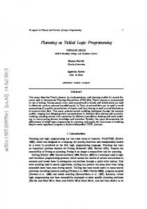
Initially, a(X) calls p(1,X) which succeeds with {X=3}, and in the continuation p(Y,Z) is called (Fig. 1(a)). The call to p(Y,Z) then checks if there are more specific subgoals being evaluated and it finds p(1,X). The subgoal frame for p(1,X) is thus marked as a consumer subgoal frame and its producer subgoal field is set to point to the subgoal frame for p(Y,Z). Next, the choice point for p(1,X) is transformed from a generator node to a retroactive node, which amounts to pruning p(1,X)’s current evaluation by updating the continuation alternative choice point field to a pseudo-instruction called retroactive resolution (Fig. 1(b)). Upon backtracking, this instruction will allow the retroactive node to transform itself in other types of nodes, as we will see. After p(Y,Z) has completed, the evaluation backtracks to p(1,X) and, by executing the retroactive resolution instruction, it is detected that the producer

Choice Point Stack

a(X), p(Y,Z) ...

a(X)

a(X), p(Y,Z)

Choice Point Stack

Choice Point Stack

a(X)

a(X)

...

Int

Int

Int

p(1,X), p(Y,Z)

p(1,X), p(Y,Z) p(1,X) Gen

p(1,X) Ret

...

p(1,X) Loa

...

X=3

X=3

p(Y,Z)

p(Y,Z)

p(Y,Z) Gen (a)

p(Y,Z) Gen (b)

(c)

Fig. 1. The base case for external pruning

subgoal has already completed. The choice point for p(1,X) is then converted to a loader node 2 (Fig. 1(c)) in order to load from p(Y,Z) all the answers relevant to p(1,X) minus the answers previously found when the choice point was a generator node (answer {X=3} in Fig. 1), therefore avoiding repeated answers. In the previous example, the pruned evaluation of p(1,X) do not included other choice points, just the generator node for p(1,X). The following example mixes subsumptive with variant checks and introduces pruning over choice points belonging to the subsumed subgoal. :- use_variant_tabling [a/2, b/1], use_subsumptive_tabling p/2. a(X,Y) :- p(1,X), b(Y). a(X,Y) :- ... b(1). b(2).

p(1,X) :- a(_,X). p(1,X) :- b(X). p(X,Y) :- ...

The query goal to consider is ‘?- a(X,Y), p(Z,W)’ and the first part of the evaluation is illustrated in Fig. 2.

Choice Point Stack

Subgoal Frames

Dependency Frames

a(X,Y), p(Z,W) a(X,Y) Gen ... p(1,X), b(Y), p(Z,W)

a(V0,V1)

a(_,X)

top_gen

top_gen

p(1,X) Gen

...

p(1,V0)

b(Y)

top_gen

top_gen

a(_,X) Con a(_,X), b(Y), p(Z,W)

b(X), b(Y), p(Z,W) ... X=1

b(X)

Gen b(V0)

b(Y), p(Z,W) ...

b(Y)

Con

top_gen

Y=1 p(Z,W)

p(Z,W) Gen

p(V0,V1) top_gen

Fig. 2. Before external pruning over choice points belonging to the subsumed subgoal 2

At the engine level, a loader node is implemented as a consumer node but without a dependency frame, since loader nodes do not need to suspend.

Execution starts by storing generator nodes for a(X,Y) and p(1,X). Next, the first clause of p/2 is executed and a consumer node for a( ,X) is allocated. As no answers for this variant subgoal exist, a( ,X) is suspended and the execution backtracks to p(1,X). The second clause of p/2 is then executed and subgoal b(X) is called, allocating a new generator node. In the continuation, a first answer for b(X) and p(1,X) is found, {X=1}, and execution proceeds with a call to b(Y). As subgoal b(Y) is a variant of b(X), a consumer node is created and the answer {X=1} is consumed, thus generating a first answer for a(X,Y), {X=1,Y=1}. Finally, subgoal p(Z,W) is called and we proceed as in the previous example for the subsumed subgoal p(1,X). But now, as the evaluation of p(1,X) includes other choice points, a( ,X) and b(X), they should be pruned. Figure 3 shows the state of the computation after pruning. The prune action depends on the choice point type and is discussed next in more detail. Pruning Interior Nodes Interior nodes are related to normal Prolog execution and can be easily pruned by ignoring them altogether. This approach, while simple, suffers from the problem of trapped choice points. A more complex solution would involve modifications to the WAM garbage collector to collect unused space on the choice point stack. Pruning Internal Consumers The consumer node for a( ,Y) must be explicitly pruned as otherwise it might be resumed, if new answers are to be consumed, and incorrectly reactivate the pruned branch of p(1,X). For each pruned internal consumer, we must thus delete its corresponding dependency frame. Pruning Internal Generators The generator node for b(X) must be explicitly pruned as otherwise it might be incorrectly completed. For each pruned internal

Choice Point Stack a(X,Y) Gen

Subgoal Frames

Dependency Frames

a(V0,V1)

b(Y)

top_gen

top_gen

a(X,Y), p(Z,W) ...

p(1,X) Ret

p(1,X), b(Y), p(Z,W)

p(V0,V1) a(_,X) top_gen

X=1 b(Y), p(Z,W)

b(X) ...

Y=1 b(Y)

Ret

p(Z,W) p(Z,W) Gen

Fig. 3. After external pruning over choice points belonging to the subsumed subgoal

generator, we must thus remove its corresponding subgoal frame from the subgoal frames stack and alter its state to pruned. Generally, when pruning internal generators, we have two situations: (i) the generator does not have consumers that are external to the computation of the subsumed subgoal; or (ii) the generator has external consumers. The former situation does not introduce any problem, but the latter origins orphaned consumers. In our example, the consumer node for b(Y) is external to the evaluation of p(1,X) and when pruning b(X), b(Y) becomes orphan. Usually, a pruned generator is called again, during the evaluation of the subsuming subgoal, and before the computation reaches any of the orphaned consumers. Once reactivated, the subgoal frame for the pruned generator is pushed again into the top of the subgoal frame stack and its state altered to evaluating. Then, the new generator node starts by consuming the previously generated answers and only then executes the program clauses. Orphaned Consumers To deal with orphaned consumers, we use the same strategy as for subsumed subgoals and transform them into retroactive nodes. Upon backtracking, they then become either: (i) a loader node, if the pruned generator was reactivated and has completed; (ii) a consumer node, if the pruned generator was reactivated but has not completed yet; or (iii) a generator node, if the pruned generator was not reactivated until then. This latter situation only occurs in variant-based tabling, since in subsumption-based tabling, when the subsuming call is executed it will necessarily either call the same or a more general subgoal, reactivating a new producer for the orphaned consumers. By default, orphaned consumers always keep their frames on the dependency frame stack. The frame is only removed if the retroactive node turns into a loader or a generator node. If the retroactive node turns again into a consumer node, lazy removal of dependency frames allows us to avoid removing and allocating a new frame and the potentially expensive operation of inserting it on the dependency frame stack in the correct order (ordered by choice point address). Lost Consumers A lost consumer is a retroactive node that will not be resumed through standard tabled evaluation, i.e., through backtracking or through answer resolution. When a lost consumer is not resumed, we might lose answers and incorrectly detect completion. As we will see next, to avoid that, we must ensure that all retroactive nodes are always resumed. While in the example of Fig. 3, both p(1,X) and b(Y) will be resumed by means of backtracking, this may not be always the case. Consider, for example, the program on Fig. 4 and the query goal ‘?- a(X,Y)’. In this example, when the subsuming call p(X,Y) is executed, the generator node b(1,X) will be pruned and the external consumer b(1,Y) (the center node in the gray oval box) will be turned into a retroactive node and became a lost consumer. Notice that b(1,Y) will be resumed neither trough backtracking, since it is not on the current branch, nor through answer resolution, since its pruned generator will not be reactivated.

:- use_variant_tabling [a/2, b/2]. :- use_subsumptive_tabling p/2. a(X,0) :- p(1,X). a(0,Y) :- b(1,Y). a(X,Y) :- p(X,Y). b(1,Y) :- a(_,Y). b(2,1). p(X,Y) :- b(X,Y).

Dependency Frames

a(X,Y) Y=0 p(1,X)

p(1,X)

X=0 b(1,Y)

top_gen

p(X,Y)

pruned by b(1,X) X=1 a(_,X)

b(1,Y) b(X,Y)

a(_,Y)

top_gen X=2 Y=1 true

a(_,Y) top_gen

Fig. 4. A lost consumer after an external pruning

Hence, when later the computation backtracks to a(X,Y) to attempt completion, b(1,Y) still remains as a retroactive node. Clearly, to correctly detect completion, we must resume it in order to generate the answers {X=0,Y=0} and {X=0,Y=1}, as otherwise they will be lost. Therefore, to ensure that all retroactive nodes are resumed, we extended the completion operation to, while traversing the dependency frame stack checking for new answers, also check for retroactive nodes, and resume the corresponding consumer node in both cases. A more tricky situation may occur when a pruned subsumed subgoal R is also a leader node3 . In such situations, R will not attempt completion and we will not be able to use the completion operation, as described above, to resume any potential lost consumer. Instead, when resuming the computation in R, if R is to be transformed into a loader node (this means that R is a pseudo-leader since no dependencies to upper nodes exist), we also traverse the dependency frame stack looking for younger retroactive nodes with unconsumed answers and, when that is the case, execution is first resumed in those nodes. With these two simple extensions, our strategy is able to ensure that all retroactive nodes are always resumed.

Frontier Node A frontier node is a choice point that is external to the computation of a subsumed subgoal R but that is chained to a choice point that is internal to the computation of R. In the example of Fig. 2, the choice point of b(Y) is a frontier node. In order to avoid execution to step into the pruned branch of a subsumed subgoal R upon backtracking, in general, a frontier node must be updated and linked to R. In the example of Fig. 3, the choice point of b(Y) is linked to p(1,X). However, for cases where the subsumed subgoal appears outside the branch of the subsuming subgoal, there is no need to update the frontier node. This is safe, because the branch including the subsumed subgoal will only be resumed on consumers during completion and thus no backtracking to previous choice points will occur as they were fully explored before. 3

The youngest generator node which does not depend on older generators is called the leader node. A leader node defines the next completion point.

3.2

Internal Pruning

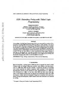
Internal pruning occurs when the subsuming subgoal S is internal to the evaluation of the subsumed subgoal R. In this type of pruning we want to keep one part of R running, the one that computes S. Our approach involves computing S using local scheduling 4 [7], but without returning answers to the environment of R, as it has been pruned. Instead, we jump directly to the choice point of R, which was transformed into a retroactive node, and resume the computation there in order to consume the matching answers found by S. When resuming the retroactive node for R, it can become either: (i) a loader node, if S has completed; or (ii) a consumer node, if S has not completed because it is not the leader node, i.e., the leader node is above R. Notice that, when the completion operation is later attempted at the leader node, the computation can still be resumed, as usual and without any special handling, at R or at the internal consumers of S, until no unconsumed answers are available. Moreover, the effects of pruning involving internal generators and external consumers discussed for external pruning, still apply to internal pruning. Our engine also supports multiple internal pruning. Consider, for instance, that a subgoal R1 calls recursively internal subgoals R2 , .., Rn until a subgoal S is called that subsumes R1 , R2 , ..., Rn . In such cases, we ignore all intermediate subgoals and answers are only pushed from S to R1 , the top subgoal. For an example, consider the query goal ‘?- p(1,X)’ and the following program: :- use_subsumptive_tabling p/2. p(1,X) :- p(2,X). p(2,X) :- p(X,_). p(X,Y) :- ....

Execution starts by storing generator nodes for p(1,X) and p(2,X), and then p(2,X) calls p(X, ) that subsumes both p(1,X) and p(2,X). Pruning is done between the top subsumed subgoal p(1,X) and the subsuming subgoal p(X, ) and the node for p(2,X) is ignored (Fig. 5(a)). The choice point for p(1,X) is transformed into a retroactive node and execution proceeds by applying local scheduling to evaluate p(X, ) (Fig. 5(b)). Later, if p(X, ) completes, the computation is resumed at p(1,X) and the retroactive node is transformed into a loader node, thus loading the matching answers from p(X, ). If p( ,X) could not complete because it is not the leader node, the evaluation still resumes at p(1,X) and the retroactive node is transformed into a consumer node, and for that it allocates a new dependency frame and inserts it in the proper order in the dependency frame stack. 4

Local scheduling is a scheduling strategy that tries to evaluate subgoals as independently as possible. The key idea is that whenever new answers are found, they are added to the table space as usual but execution fails. Hence, answers are only returned when all program clauses for the subgoal at hand were fully explored.

Choice Point Stack

p(1,X) ... p(2,X)

Choice Point Stack

p(1,X)

p(1,X) Gen

p(2,X) Gen

p(1,X) Ret

p(X,_)

p(2,X)

... p(X,_) Gen

p(X,_)

Local Scheduling

(a)

p(X,_) Gen

(b)

Fig. 5. Multiple internal pruning

4

Implementation Details

In this section, we describe implementation details worthy of note. First, we will describe some other topics related to pruning, next we present how the table space is organized, and, then, we give a brief overview of the algorithm used to search for subsumed subgoals.

From Consumers to Generators In order to be able to transform a consumer node into a retroactive node and then into a generator node, all consumer choice points are allocated, by default, as generator choice points. We are studying a more sophisticated solution that will uniformize the choice point representation of tabled nodes in order to simplify this problem.

External or Internal Each subsumptive subgoal frame was extended with two new fields: start code and end code, that initially are standard WAM variables. The start code field is bound to an arbitrary value when the subgoal starts executing and unbound when the subgoal backtracks, therefore allowing us to easily detect if the subgoal is in the current branch. The end code field is bound when a new answer is found, i.e., when the code has reached the end of a program clause, thus allowing us to easily detect if a pruned subgoal is external or internal. To reconstruct the dependency tree of generators and consumers, we extended both subgoal and dependency frames with a new top gen field (see Figs 2 and 3). When a new frame is created, this field is set to point to the subgoal frame corresponding to the generator node whose code is in execution, if any. This subgoal frame is represented by a global variable that is updated when a new generator is called or when it reaches the end of a program clause. Dependency frames save the value of this global variable in order to correctly restore it when a consumer node is resumed. In order to detect if a subgoal S is external or internal to another subgoal R, the top gen links are traversed until: (i) R is reached and, in this case, S is internal; or (ii) we reach a subgoal older than R and, in this case, S is external.

Table Space In our subsumptive engine, all answers for a tabled predicate are stored in a Single Time Stamped Trie (STST) that is common to all subgoals calls for the predicate. This approach reduces memory usage, allows easy sharing of answers between different subgoals and, in particular, allows us to efficiently load answers from subsumed/subsuming subgoals. The STST keeps a time stamp for the last answer inserted and each subgoal frame keeps a time stamp for the last answer generated or consumed. This time stamps are then used to easily compute the answers to be considered when pruning a subsumed subgoal. This approach also allows reusing the answers on the STST when a new subgoal is called. As an example, consider that two unrelated (no subsumption involved) subgoals S1 and S2 are fully evaluated. If a subgoal S is then called, it is possible that some of the answers on the STST match S even if S neither subsumes S1 nor S2 . Hence, instead of eagerly running the predicate clauses, we start by loading the matching answers already on the STST, which can be enough if, for example, S gets pruned by a cut. While this approach has some advantages, it can lead to redundant computations if later, when running the program clauses, S generates more general answers than the ones initially loaded. Searching Subsumed Subgoals Each subgoal trie node was extended with a new field called in eval which stores the number of subgoals, represented below the node, that are in evaluation. The subgoal trie path is incremented or decremented when the subgoal enters or exists the computation, respectively. Our algorithm for searching subsumed subgoals then uses this field to quickly discard irrelevant trie branches as it descends the trie. The search is done by matching the subgoal arguments through backtracking along the subgoal trie. On a successful match, the algorithm stores a continuation for an alternative node before descending into the next trie level. If a match fails, a continuation is popped from the continuation stack and the state of the computation is restored (bindings and the trie node). The matching works by the following rules. A nonvariable term argument must always match with a non-variable trie symbol. Unbound variable term arguments can match any trie symbol and are bound to the symbol before descending. When a variable term bounds to a trie variable, it must always match against the same trie variable on the following matches.

5

Experimental Results

In this section, we present some experimental results comparing our new RCS proposal with traditional call subsumption. The environment for our experiments was an Intel Core(TM) 2 Quad 2.66 GHz with 4 GBytes of memory and running the Linux kernel 2.6.31 with YapTab 6.0.3 and XSB Prolog 3.2. First, we measured the RCS overhead for programs that do not take advantage of it, i.e., programs that never call more general subgoals after specific ones, and for that we used a set of benchmark programs downloaded from the XSB Prolog repository5 with different configurations of data (see Table 1). 5

http://xsb.cvs.sourceforge.net/viewvc/xsb/xsbtests

Program/Data binary tree chain right first grid pyramid binary tree chain left last grid pyramid binary tree double last chain binary tree samegen chain Average Table 1. RCS running times

RCS 170 2,900 14,456 11,520 146 3,068 13,356 3,260 952 2,912 8,272 44

CS/RCS XSB/RCS 0.94 0.96 0.99 1.10 1.18 1.20 1.00 1.01 0.93 0.96 0.93 1.24 1.00 1.28 1.08 0.90 0.94 1.03 0.90 1.41 0.97 1.20 1.18 0.64 1.00 1.08 on programs that do not benefit from it

Table 1 shows the running time, in milliseconds, for YapTab using RCS (column RCS), and its ratio compared with traditional call subsumption for both YapTab (column CS/RCS) and XSB Prolog (column XSB/RCS). Our results show that, for this set of programs, RCS support adds a very small overhead to running time when compared with traditional call subsumption, and for some programs it can even run faster, probably due to cache behavior effects. Next, we tried some benchmarks where RCS was expected to perform better. We used a path/2 program, left and doubly recursive variants, to compute the query goal ‘?- path(X,1)’ and also experimented a reach/2 program with three different transition relation graphs used in model-checking applications. From Table 2, we can observe that for some path/2 benchmarks, RCS performs worse, possibly because the time saved by pruning evaluation branches does not pay the incurred overhead in traversing the new STST table organization to collect relevant answers. For the model-checking benchmarks, RCS performance is notoriously better than traditional call subsumption, with speedups reaching 2.18 for YapTab and 4.33 for XSB. For these benchmarks, the performance impact of using the STST is much smaller when compared to the time saved by pruning evaluation branches of subsumed subgoals.

6

Conclusions and Further Work

We have presented a new tabling extension called Retroactive Call Subsumption that supports full sharing of answers between subsumptive subgoals, regardless of the order in which they are called, and we have described the main concepts and operational challenges of its design in the context of the YapTab system. Initial experiments comparing our proposal with traditional call subsumption semantics, showed low overheads when executing standard programs and good results when applied to tabled programs that can benefit from it. Further work involves refining the system, testing it against more real-world applications, and studying the impact on performance and memory usage of new data structures, like the Single Time Stamped Trie.

Program/Data RCS CS/RCS XSB/RCS binary tree 156 1.18 1.18 chain 44 1.00 1.18 left first grid 40 1.20 1.40 pyramid 200 0.92 0.96 binary tree 784 1.62 1.46 chain 2,916 0.95 1.24 double first grid 2,132 0.97 1.30 pyramid 12,004 1.01 1.19 iproto 2,244 1.54 2.77 reach first leader 3,152 1.92 3.82 sieve 19,997 1.94 1.96 iproto 2,300 1.51 2.77 reach last leader 3,128 1.94 4.33 sieve 17,693 2.18 2.97 Average 1.42 2.01 Table 2. RCS running times on programs that are expcted to benefit from it

As argued by Johnson et al. [3], for some programs it may be useful to lose some goal directness by means of call abstraction and, instead of calling a goal G, we may decide to call a more general goal G0 and then reuse the answers from G0 to solve G. Our implementation already includes all the machinery necessary to do that, which makes it a good framework to further support call abstraction by devising various analysis techniques of call patterns.

References 1. Chen, W., Warren, D.S.: Tabled Evaluation with Delaying for General Logic Programs. Journal of the ACM 43(1) (1996) 20–74 2. Rao, P., Ramakrishnan, C.R., Ramakrishnan, I.V.: A Thread in Time Saves Tabling Time. In: Joint International Conference and Symposium on Logic Programming, The MIT Press (1996) 112–126 3. Johnson, E., Ramakrishnan, C.R., Ramakrishnan, I.V., Rao, P.: A Space Efficient Engine for Subsumption-Based Tabled Evaluation of Logic Programs. In: Fuji International Symposium on Functional and Logic Programming. Number 1722 in LNCS, Springer-Verlag (1999) 284–300 4. Costa, J., Rocha, R.: Global Storing Mechanisms for Tabled Evaluation. In: International Conference on Logic Programming. Number 5366 in LNCS, Springer-Verlag (2008) 708–712 5. Rocha, R., Silva, F., Santos Costa, V.: On applying or-parallelism and tabling to logic programs. Theory and Practice of Logic Programming 5(1 & 2) (2005) 161–205 6. Warren, D.H.D.: An Abstract Prolog Instruction Set. Technical Note 309, SRI International (1983) 7. Freire, J., Swift, T., Warren, D.S.: Beyond Depth-First: Improving Tabled Logic Programs through Alternative Scheduling Strategies. In: International Symposium on Programming Language Implementation and Logic Programming. Number 1140 in LNCS, Springer-Verlag (1996) 243–258