A Modified Approximation of 2D Gaussian Smoothing Filters for Fixed-Point Platforms Sami Khorbotly
Firas Hassan
Dept. of Elec. & Comp. Eng. & Comp. Sc. Ohio Northern University Ada, Ohio, USA
[email protected]
Dept. of Elec. & Comp. Eng. & Comp. Sc. Ohio Northern University Ada, Ohio, USA
[email protected]
Abstract - Gaussian smoothing filters are commonly used in various image processing applications to reduce the noise level in an image. The filters are particularly popular in edge detection algorithms because of their ability to smooth false edges and improve the edge detection performance. When implemented on a fixed-point computational platform, the filter coefficients are rounded and the implemented filter becomes a rounded approximation of the original one. In those implementations, system designers must balance between signal integrity and the hardware size they can afford in a particular design. In this work, we suggest a new “modified” method to approximate the coefficients of a 2D Gaussian filter. When implemented on a Field Programmable Gate Array (FPGA), the modified approximation filter is shown to generally deliver higher signal quality than its traditional “rounded” counterpart without any increase in the required resources.
I.
INTRODUCTION
The fields of image processing and computer vision are continuously gaining increased attention in applications including robotics, automation, quality control, and security systems. Among the many image processing procedures, edge detection is seen by many as the first essential step in any type of image analysis. It is used to separate the image into object(s) and background. The performance of an edge detection operator is defined as its ability to locate, in noisy data, an edge that is as close as possible to its true position in the image [1]. Since most edge detection operators employ differentiationbased techniques, any noise in the considered image will be dramatically amplified, resulting in unfavorable results. Therefore, in order to improve the performance of an edge detection algorithm, some type of noise reduction, or image smoothing, to a certain degree must be performed prior to the application of the edge detection operator. The amount of the employed smoothing depends on the scale and the size of the utilized filter. It has been shown that selecting a single smoothing scale that is optimal for detecting all the different edges in an image is almost impossible. As an alternative, system designers use multi-scale smoothing and edge detection operators to extract different edges at different scales that are later combined to obtain all the edges in an image.
In the current research world, the focus has been to develop the most effective edge detection algorithm with little to no attention to the computational complexity and the hardware requirements. While this can be understandable when the algorithms are implemented on personal or super computer platforms, it must be reconsidered in the case of embedded applications like portable devices or small scale robots, where the hardware size is usually a major concern. Field Programmable Gate Arrays (FPGA) are frequently used for the implementation of digital signal processing and digital image processing systems. Compared to Digital Signal Processors (DSP), FPGAs are shown to be two orders of magnitude faster and are proven to have better hardware utilization [2]. Unlike the floating-point based DSPs, FPGAs implement fixed-point mathematics which often raises accuracy issues with the realization of signal processing algorithms in finite precision hardware. As a result, it is critical for designers to select the appropriate fixed-point data format to represent their filters’ coefficients. The selection must be carefully made in a way to balance between signal integrity (larger number of bits) and hardware cost (lower number of bits). II.
GAUSSIAN SMOOTHING FILTERS
Smoothing can be achieved using various types of filters, the most common of which is the Gaussian filter discussed in this paper. The 2D Gaussian filters are commonly adopted in multi-scale edge detection techniques for three main reasons. The first reason is that when combined with a Laplacian operator, the 2D Gaussian filters are the only filters that do not create false edges as the scale increases [3]. The second reason is that Gaussian filters give the best tradeoff between localization in both spatial and frequency domains. The third reason is that Gaussian filters are the only rotationally invariant 2D filters that are separable in the horizontal and the vertical directions, which makes the convolution in the spatial domain very efficient. Among the many famous edge detection algorithms that use Gaussian smoothing are MarrHildreth detector [4] and the Canny detector [5]. While Gaussian filters are mostly used in the edge detection area, they are also commonly used in many other applications including image mosaicing [6] and tone mapping of high dynamic range images [7].
A 2D Gaussian function centered at the origin with a standard deviation σ can be described by: ݃ሺݔ, ݕሻ = ݁
ష൫ೣమ శమ ൯ మమ
.
(1)
While the function theoretically evaluates to non-zero for all values of x and y, it is a common practice to consider the function to be effectively zero for x and y values beyond three standard deviations from the mean. When an image h is smoothed by the Gaussian filter with impulse response g, the smoothed image f can be found in the frequency domain using the expression ܨሺݑ, ݖሻ = ܪሺݑ, ݖሻ × ܩሺݑ, ݖሻ
(2)
where F(u,z), H(u,z), and G(u,z) are respectively the frequency domain representations of f(x,y), h(x,y), and ݃ሺݔ, ݕሻ. Similarly, the smoothed image can be found in the spatial domain using the convolution expression ݂ሺݔ, ݕሻ = ℎሺݔ, ݕሻ ∗ ݃ሺݔ, ݕሻ .
(3)
In order to effectively compute the convolution sum shown above, the impulse response of the 2D filter ݃ሺݔ, ݕሻ must be approximated by a finite number of coefficients, commonly known as the convolution kernel, or the mask. The dimensions of the mask are usually determined based on the standard deviation (σ) of the Gaussian function. For additional smoothing, a larger value of σ must be chosen and a larger kernel is needed to accurately represent the function. In this paper, a Gaussian smoothing filter with σ=1 is considered. The 5x5 kernel corresponding to this filter can be obtained by evaluating (1) for (x,y) values between (-2,-2) and (2,2). It is worth mentioning that for this kernel, the considered finite size kernel (25 samples) accounts for 96.4% of the energy of its infinite size counterpart. An important criterion that is considered is the sum of the kernel coefficients. It is important for the implemented convolution kernel to be made of coefficients that sum up to 1 for the smoothed image to have the same average intensity as the original image. As a result, the normalized kernel is obtained by dividing each element of the original one by the sum of the 25 coefficients ݃ ሺݔ, ݕሻ = ݃ሺݔ, ݕሻ/ܰ
(4)
Where ܰ=
ଶ ௫ୀିଶ
ଶ ௬ୀିଶ
݃ሺݔ, ݕሻ.
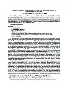
As can be expected by looking at (1) and (4), the normalized Gaussian coefficients are real numbers that are usually represented by floating point values. Fig. 1 shows the values of the 5x5 kernel corresponding to ݃ ሺݔ, ݕሻ with the coefficients rounded to the 4th decimal point.
0.0030 ۍ0.0133 ێ ێ0.0219 ێ0.0133 ۏ0.0030
0.0133 0.0596 0.0983 0.0596 0.0133
0.0219 0.0983 0.1621 0.0983 0.0219
0.0133 0.0596 0.0983 0.0596 0.0133
0.0030 0.0133ې ۑ 0.0219ۑ 0.0133ۑ 0.0030ے
Fig. 1. Normalized coefficients of a 5x5 Gaussian kernel with σ=1.
III.
FIXED-POINT IMPLEMENTATION
In this paper, the fixed-point data is represented in the (l,m) format, where l represents the number of bits used, and m represents the location of the coefficient’s least significant bit. For example, the decimal equivalent of the coefficient x3x2x1x0 in a (4,2) format is ݔଷ × 2ହ + ݔଶ × 2ସ + ݔଵ × 2ଷ + ݔ × 2ଶ while the decimal equivalent of the same coefficient in a (4,2) format is ݔଷ × 2ଵ + ݔଶ × 2 + ݔଵ × 2ିଵ + ݔ × 2ିଶ . The Fixed-Point implementation of FIR filters with powers-oftwo coefficients has been studied in [8] and [9]. Both papers approach the problem by restricting the representation of each filter coefficient to the sum of two non-zero powers-of-two. Different types of suboptimum algorithms are used to find the coefficients that minimize the error between the frequency response of the ideal floating point FIR filter and its powersof-two version. Both works target high order FIR filters of around 200 taps, which is usually not the case in 2D filters used in image processing. In our work, for the Gaussian smoothing application, each coefficient is rounded to the nearest achievable value within the available bit-width budget regardless of the number of non-zero coefficients. In order to avoid complex multiplication and division operations, the coefficient multiplications are implemented by shift and add operations. For example, if a variable v is to be multiplied by the 4-bit coefficient 0.55, the coefficient 0.55 will be rounded to its nearest 4-bit value of 0.562510≡10012 in the (4,-4) format; the multiplication of v by that coefficient will be implemented by 0.55ܽ =
9 2ଷ × ܽ + ܽ ܽ= 16 2ସ
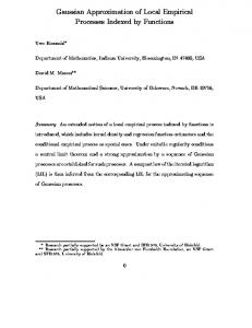
where the multiplication and the division by powers of 2 of v are respectively implemented by the hardware-friendly right shift and left shift operations. In order to implement and test the Gaussian smoothing filter on an FPGA platform, the smoothing kernel is rounded and written in various fixed-point data formats with various bit budgets. Also, it is mandated in our work that all coefficients in a kernel must be represented by the same fixed-point data format. This significantly simplifies the hardware by ensuring the same data format for intermediate signals. Fig. 2 shows the Gaussian smoothing kernel shown in Fig. 1 rounded to the (2,-4) and (6,-8) data formats.
0 ۍ 1 ێ0 0 2ସ ێ ێ0 ۏ0 1 ۍ3 1ێ 6 2଼ ێ ێ3 ۏ1
0 1 2 1 0 3 15 25 15 3
0 2 3 2 0
0 1 2 1 0
6 25 41 25 6
3 15 25 15 3
(a)
0 0ې ۑ 0ۑ 0ۑ 0ے
TABLE I. Kernel sums for various implementation formats.
1 3ې ۑ 6ۑ 3ۑ 1ے
(b) Fig. 2. The Gaussian smoothing kernel (a) data format (2,-4) (b) data format (6,-8).
IV. THE MODIFIED GAUSSIAN KERNEL When the Gaussian kernel is rounded to be written in the various fixed-point formats, the following two different forms of errors are introduced: 1.
2.
Quantization Errors: a result of the difference between the coefficients’ original and rounded values. This error has an upper limit that is directly related to the available bit budget and can be reduced at the expense of increasing the coefficients’ bit-widths. Average intensity error: while designers create Gaussian kernels with a unity sum, it is extremely unlikely that the rounded coefficients will maintain this property. Table I shows the sums of our example kernel when rounded to different fixed-point formats. The convolution by a Gaussian kernel with a non-unity sum results in a smoothed image with a different average intensity (lighter/darker) than the original one. This error is a random error that cannot be estimated and is not related to any design parameter.
While the algorithms presented in [8] and [9] are developed to obtain the powers-of-two filter with the closest frequency response to the original one, maintaining a unity sum of the filter coefficients was not taken into consideration and the average intensity error was not taken into account. This error becomes a critical issue in image processing applications especially in applications like edge detection where the smoothing filter may be applied multiple times resulting in a significant offset in the brightness/darkness of the smoothed image. In order to account for both types of error, rather than finding the coefficients that will best approximate the frequency response of the filter, our goal is to obtain the powers-of-two filter that will maximize the SNR of the filtered image. The SNR is calculated with the noise being the difference between the image filtered by the powers-of-two filter and the one filtered by the reference filter. To maximize the SNR of the fixed-point Gaussian kernel we suggest all the kernel’s coefficients to be rounded to their nearest achievable value, except the center coefficient which value is selected to achieve a unity sum.
Format
Sum
(2,-4)
0.9375
(3,-5)
0.9063
(4,-6)
0.9688
(5,-7)
1.0391
(6,-8)
0.9883
(7,-9)
1.0059
(8,-10)
1.0020
For example, the rounded (2,-4) Gaussian smoothing kernel shown in Fig. 2(a) has a sum of 0.9375. The unity sum is restored in the modified version by changing the value of the center coefficient from
ଷ
ଶర
to
ସ
ଶర
. Similarly, the center
coefficient in the rounded (6,-8) kernel shown in Fig. 2(b) will be changed from
ସଵ ଶఴ
to
ସସ ଶఴ
to obtain the modified version.
While this modification increases the quantization error by deviating the center coefficient from its nearest achievable value, it totally eliminates the random-nature average intensity error and reduces the problem to dealing with only one type of error that is easier to estimate and handle. As mentioned earlier, 2D Gaussian smoothing filters are separable and can be implemented using a pair of 1D filters. In this setup, one filter v operates on the image data in the vertical direction and another filter h operates on the output of v in the horizontal direction. The equivalent 2D filter w is obtained by × ்ݒ = ݓℎ Following our approach, the separation of the 2D filter can become problematic. Suppose the considered 2D Gaussian kernel w is implemented in the (5,-7) format. The separated 1D filters v & h can be written in the (3,-4) and (2,-3) formats as follows: 1 v = 3 [0 2 3 2 0] 2 ( 2, −3) 1 h = 4 [1 4 6 4 1] 2 (3, −4)
Since the filter v has a non-unity sum of coefficients, its center coefficient must be modified from
ଷ
ଶయ
to
ସ
ଶయ
to eliminate the
average intensity error. Following the modification, the resulting 2D kernel, shown in fig. 3(a), has lost its Gaussian shape and some of its Gaussian properties particularly the rotational invariance. On the other hand, the same filter designed and modified in 2D, shown in fig. 3(b), has maintained its Gaussian shape and its rotational invariance. For this reason, while totally aware that a 2D Gaussian filter is separable, it was decided to design and modify the Gaussian kernel in 2D rather than designing and modifying a pair of 1D filters.
0 ۍ 1 ێ0 0 2 ێ ێ0 ۏ0
2 8 12 8 2
4 16 24 16 4
2 8 12 8 2
0 0ې ۑ 0ۑ 0ۑ 0ے
2 8 13 8 2
0 2ې ۑ 3ۑ 2ۑ 0ے
(a) 0 ۍ2 1ێ 3 2 ێ ێ2 ۏ0
2 8 13 8 2
3 13 16 13 3 (b)
(a)
Fig. 3. The Gaussian kernels (a) designed using two 1D filters (b) designed as a 2D filter
V. EVALUATION CRITERION In order to quantitatively evaluate and compare the errors associated with our modified kernels and the rounded (but not modified) ones, the famous “Lena” image shown in Fig. 4(a) is used as a test case. A 512x512 pixels gray scale version of the image is obtained and used in the rest of the work. To obtain a reference, ideally smoothed version of the image, filtering was performed in the frequency domain using the Matlab computing environment. Filtering in the frequency domain is accomplished by implementing the following steps: 1. Use the Fourier Transform to obtain a 512x512 matrix representation of the image in the frequency domain. 2. Use the Fourier Transform to obtain a 512x512 matrix representation of the Gaussian smoothing filter (with σ=1) in the frequency domain. 3. Perform an element-by-element multiplication of the matrices in steps 1 & 2 to obtain a 512x512 matrix representation of the frequency domain smoothed image. 4. Use the Inverse Fourier Transform to obtain a 512x512 matrix representing the spatial domain filtered version of the image. The image obtained in step 4 is shown in Fig. 4(b) and is the reference smoothed image to which the performances of the various smoothing kernels are compared. This image is considered the reference because the Gaussian function used to smooth it was represented by 512x512 coefficients and was not limited by a smaller finite size window (like the spatial domain kernels). Also, since the computation is performed in Matlab, a floating-point mathematics tool, coefficients are accurately represented without quantization errors. To compare the performances of the various smoothing kernels on the considered image, the Signal to Noise Ratio (SNR) is adopted. With the signal being the reference image s, the signal power S can be obtained using the formula ܵ=
ହଵଶ ௫ୀଵ
ହଵଶ ௬ୀଵ
ݏଶ ሺݔ, ݕሻ.
Similarly, if a smoothed image im1, obtained using a particular smoothing kernel, is to be compared to s, the noise power N can be obtained using the formula:
(b) Fig. 4. Two versions of the “Lena” image. (a) Original. (b) Smoothed with a Gaussian filter of σ=1 in the frequency domain.
ܰ=
ହଵଶ ௫ୀଵ
ହଵଶ
ሺݏሺݔ, ݕሻ − ݅݉1ሺݔ, ݕሻሻଶ
௬ୀଵ
and the SNR in dB can be obtained using the formula ܴܵܰ = 10݈݃
ௌ
ே
.
VI. HARDWARE IMPLEMENTATION The FPGA implementation of the smoothing filter is carried out on a microEnableIV fullx1 module [10] from Silicon Software, GmbH [11]. The module is a Peripheral Component Interconnect Express (PCIe) based board with a Camera Link interface for image and video acquisition. It also includes two Spartan 3E FPGAs from Xilinx, 256 MB DDR-RAM onboard, and additional FPGA on-board memory for preprocessing. It also supports numerous add-on boards for additional connectivity options. The PCIe nature of the module makes it simple to interface to a Personal Computer (PC) which significantly simplifies the FPGA programming task and makes it easy to also display the system’s output on the PC screen. In order to implement the multiple versions of the Gaussian smoothing filter on the microEnable module, Visual Applets 1.2 [12], also from Silicon Software, GmbH [11], was used. Visual Applets is a block-based graphical programming tool designed for digital image processing applications. The
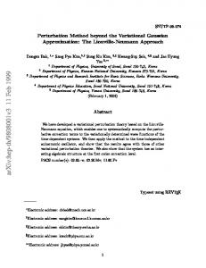
VII. RESULTS When the test system is implemented in hardware, the Gaussian smoothing kernel must be implemented together with a frame grabber that reads the frames from a camera and eventually displays them on the PC screen. In the first test, the frame grabber was implemented by itself (no smoothing filter) to determine the amount of hardware resources dedicated to it. Three various hardware resources are measured and reported, namely the number of internal RAMs, the number of logic elements, and the number of flip flops. The frame grabber’s implementation was achieved using 4 internal RAMs, 2637 logic elements, and 1980 flip flops. When the Gaussian smoothing kernel is added to the design, the kernel was implemented using different bit configurations where the number of bits representing the filter’s coefficients was varied from 2 to 8 bits. The hardware resources needed for both the rounded and the modified versions for each of the different bit configurations are shown in Table II. The results show that number of RAMs remains constant in all the configurations. This is not surprising since all the implemented designs used 5x5 kernels. A larger kernel size would result in additional RAM usage. Also, as expected, the number of used logic elements and flip flops grows with the increase in the number of bits. This is a result of the additional shift and add operations needed to perform the additional multiplications. Comparing the modified and the rounded versions of each bit format, it is clear that the modified version does not require any additional hardware resources. Contrarily, the modified version is likely to be implemented with less logic elements and flip flops compared to the rounded version depending on the binary representation of the modified center coefficient. To compare the smoothing quality of the rounded and the modified versions of the Gaussian approximation for each of the various bit configurations, the image “Lena” shown in Fig. 4(a) was smoothed using the various implementations. The output images were compared to the reference smoothed image shown in Fig. 4(b) and the SNR values are shown in Fig. 5. As can be seen in the Figure, the SNR of the images smoothed with the modified kernels monotonically improves as the number of available bits increases, making it easier for a designer to balance the quality vs cost trade-off. The same cannot be said about images smoothed with the rounded kernel where a 3 bit kernel results in a lower smoothing quality than a 2 bit kernel. This low performance of the 3 bit rounded smoothing kernel can be explained by the significant deviation of the sum of that kernel from the unit value (see table I). Also looking at the same figure the (7,-9) rounded kernel outperforms its modified counterpart by around 2dB because the sum of the rounded kernel in that particular format is extremely close to the unit value.
Table II. Hardware resources used to implement various configurations of the Gaussian smoothing filters (with frame grabber)
Format (2,-4) (3,-5) (4,-6) (5,-7) (6,-8) (7,-9) (8,-10)
Int. RAMs Mod Round 12 12 12 12 12 12 12 12 12 12 12 12 12 12
Logic Elem. Mod Round 3239 3257 3421 3441 3683 3683 3829 3919 4363 4363 4561 4619 4955 4985
Flip Flops Mod Round 2446 2446 2448 2448 2487 2487 2489 2493 2495 2495 2499 2501 2503 2503
50 45 40 SNR (dB)
programmers use a graphical user interface to select the configurable blocks from the provided libraries of hardware based operators covering the major image processing functions and interconnect them to implement their particular systems. Visual Applets converts the graphical design to a hardware applet that is synthesized using Xilinx tools on the target FPGA device.
35 30 25 Rounded Modified
20 15 2
3
4
5 n (bits)
6
7
8
Fig. 5. The performance of both rounded and modified kernels on the test image for various bit formats.
However, the modified kernels outperform the rounded ones for all the other bit configurations by up to 19dB. VIII. CONCLUSION In this paper, a modified fixed-point approximation of 2D Gaussian smoothing filters is presented. The approach is much simpler than the methods described in [8] and [9]. It designs the 2D filter directly without separating the filter into two 1D filters. The modified approximation is shown to achieve a higher performance in most bit configurations, especially with lower bit budgets. The modified approximation is also shown to have an improved performance as the bit budget is increased. The suggested modified approximation does not require any additional resources as it can be implemented using the same, if not less hardware compared to the rounded version. REFERENCES [1] M. Basu, “Gaussian based edge detection methods—A survey,” IEEE Transactions on systems, man, and cybernetics—Part C: Applications and reviews, vol. 32, No. 3, August 2002. [2] F. Krach, B. Frackelton, J. Carletta, & R. Veillette, “FPGA-based implementation of digital control for a magnetic bearing,” IEEE American Control Conference. June 2003. [3] A. Yuille & T. Poggio, “Scaling theorems for zero-crossings,” IEEE Transactions on Pattern Analysis and Machine Intelligence, vol. PAMI-8, Jan. 1986.
[4] D. Marr and E. Hildreth, “Theory of edge detection,” Proceedings of the Royal Society of London. Series B, Biological Sciences vol. 207, No. 1167, Feb. 1980. [5] J. Canny, “A computational approach to edge detection,” IEEE Transactions on Pattern Analysis and Machine Intelligence, vol. PAMI-8, June 1986. [6] P. Burt, & E. Adelson, “A multiresolution spline with application to image mosaics,” ACM Transactions on Graphics, vol. 2, No. 4, Oct. 1983. [7] E. Reinhard, M. Stark, P. Shirley, & J. Ferwarda,” Photographic tone reproduction for digital images,” Proc. of the Conference on Computer Graphics and Interactive Techniques, 2002. [8] Y. C. Lim, S. R. Parker,” FIR filter design over a discrete powers-of-two coefficient space,” IEEE transaction on acoustics, speech, and signal processing, vol. 31, no. 3, June 1983. [9] Q. Zhao and Y. Tadokoro,” A simple design of FIR filters with powers-oftwo coefficients,” IEEE transactions on circuits and systems, vol. 35, no. 5, May 1988. [10] http://www.silicon-software.com/microenable4.html [11] www.silicon-software.com [12] http://www.silicon-software.com/visualapplets.html