Mar 6, 2015 - cones of arbitrary basis [Franco and Boyer, 2009]. ...... We are grateful to Edmond Boyer, François Faure and Stan Borkowski for fruitful ...
QuickCSG: Arbitrary and Faster Boolean Combinations of N Solids Matthijs Douze, Jean-S´ebastien Franco, Bruno Raffin
To cite this version: Matthijs Douze, Jean-S´ebastien Franco, Bruno Raffin. QuickCSG: Arbitrary and Faster Boolean Combinations of N Solids. [Research Report] RR-8687, Inria - Research Centre Grenoble – Rhˆone-Alpes; INRIA. 2015.
HAL Id: hal-01121419 https://hal.inria.fr/hal-01121419 Submitted on 6 Mar 2015
HAL is a multi-disciplinary open access archive for the deposit and dissemination of scientific research documents, whether they are published or not. The documents may come from teaching and research institutions in France or abroad, or from public or private research centers.
L’archive ouverte pluridisciplinaire HAL, est destin´ee au d´epˆot et `a la diffusion de documents scientifiques de niveau recherche, publi´es ou non, ´emanant des ´etablissements d’enseignement et de recherche fran¸cais ou ´etrangers, des laboratoires publics ou priv´es.
QuickCSG: Arbitrary and Faster Boolean Combinations of N Solids
March 2015 Project-Teams Morpheo, Moais
ISSN 0249-6399
RESEARCH REPORT N° 8687
ISRN INRIA/RR--8687--FR+ENG
Matthijs Douze, Jean-Sébastien Franco, Bruno Raffin
QuickCSG: Arbitrary and Faster Boolean Combinations of N Solids
Matthijs Douze, Jean-Sébastien Franco, Bruno Ra�n Project-Teams Morpheo, Moais Research Report
Abstract:
n° 8687 � March 2015 � 36 pages
While studied over several decades, the computation of boolean operations on
polyhedra is almost always addressed by focusing on the case of two polyhedra. For multiple input polyhedra and an arbitrary boolean operation to be applied, the operation is decomposed over a binary CSG tree, each node being processed separately in quasilinear time. For large trees, this is both error prone due to intermediate geometry and error accumulation, and ine�cient because each node yields a speci�c overhead. We introduce a fundamentally new approach to polyhedral CSG evaluation, addressing the general N-polyhedron case. We propose a new vertex-centric view of the problem, which both simpli�es the algorithm computing resulting geometric contributions, and vastly facilitates its spatial decomposition.
We then embed the entire problem in a single
KD-tree, speci�cally geared toward the �nal result by early pruning of any region of space not contributing to the �nal surface. This not only improves the robustness of the approach, it also gives it a fundamental speed advantage, with an output complexity depending on the output mesh size instead of the input size as with usual approaches. Complemented with a task-stealing parallelization, the algorithm achieves breakthrough performance, one to two orders of magnitude speedups with respect to state-of-the-art CPU algorithms, on boolean operations over two to several dozen polyhedra. The algorithm is also shown to outperform recent GPU implementations and approximate discretizations, while producing an exact output without redundant facets.
Key-words:
CSG, Polyhedra, boolean operations
This is a note
This is a second note
RESEARCH CENTRE GRENOBLE – RHÔNE-ALPES
Inovallée 655 avenue de l’Europe Montbonnot 38334 Saint Ismier Cedex
QuickCSG: combinaison booléenne arbitraire et rapide de N solides
Résumé :
Quoique étudié depuis des décennies, le calcul d'opérations booléennes sur des
polyèdres est quasiment toujours fait sur deux opérandes. Pour un plus grand nombre de polyèdres et une opération booléenne arbitraire à e�ectuer, l'opération est décomposée sur un arbre binaire CSG (géométrie constructive), dans lequel chaque n÷ud est traité séparément en temps quasi-linéaire.
Pour de grands arbres, ceci est à la fois source d'erreurs, à cause des calculs
géométriques intermédiaires, et ine�cace à cause des traitements super�us au niveau des n÷uds. Nous introduisons une approche fondamentalement nouvelle qui traite le cas général de N polyèdres. Nous proposons une vue du problème centrée sur les sommets, ce qui simpli�e l'algorithme et facilite sa décomposition spatiale. Nous traitons le problème dans un seul KD-tree, qui est dirigé vers le résultat �nal, en élaguant les régions de l'espace qui ne contribuent pas à la surface �nale. Non seulement ceci améliore la robustesse de l'approche mais ça lui donne un avantage en vitesse, car la complexité dépend plus de la taille de la sortie que celle d'entrée. En la combinant avec une parallélisation basée sur du vol de tâche, l'algorithme a des performances inouïes, d'un ou deux ordres de grandeur plus rapide que les algorithmes de l'état de l'art sur CPU et GPU. De plus il produit un résultat exact, sans aucune primitive géométrique super�ue.
Mots-clés :
Opérations booléennes, polyèdres
QuickCSG
Figure 1:
3
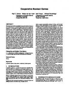
Intersection of 6 Buddhas with the union of 100,000 spheres (total 24 million triangles).
Computed in 8 seconds on a desktop machine.
1
Introduction
Solid modeling using boolean operations is an emblematic problem in computer graphics and computational geometry, almost as old as these research topics themselves. It has found its way in every solid modeler in the industry, whether applied to model design for aviation, transportation, manufacturing, architecture, or entertainment. It is also an ubiquitous building block and subject of interest for many �elds of research, including computer graphics, computer vision, robotics, virtual reality, and generally any topic where geometric models of subjects of interest are to be manipulated, constructed, truncated or combined. Since the �rst introduction of boundary representations (B-Rep) [Baumgart, 1974], the problem has received considerable attention and been the subject of extensive work over more than 40 years.
It is all the more striking that, despite the many existing algorithms and variants
in this huge corpus, the vast majority of algorithms generally rely on a common principle and canvas found in the earliest formalizations of the problem [Requicha and Voelcker, 1985, Laidlaw et al., 1986].
First and foremost, boolean B-Rep merging algorithms are most often
written for the case of two solids. Second, the computation is most commonly divided in three stages: an initial
subdivision
stage, where the boundaries of both objects are split in two com-
ponent groups along their intersection with the other object's boundary. A
classi�cation
stage
follows, where each group is classi�ed as belonging inside or outside the other object. In the �nal
reconstruction
stage, the relevant primitives are gathered and connected to build the �nal model
in accordance to the boolean expression. Note that the subdivision and classi�cation require to intersect and situate all primitives of an object's boundary with respect to the primitives of the other object's boundary, which if done naively leads to impractical quadratic-time algorithms. Thus, a third common aspect of most algorithms is the use of spatial decomposition structures, often hierarchical, to enable sublinear
O(log n) access to each object's primitives.
The construction
of this data structure usually becomes the bottleneck of the algorithm, giving it its typically quasilinear time complexity (where
d
O(n logd n)
in the number of input primitives [Hachenberger et al., 2007]
is a constant).
In a majority of the use cases, solids are built using several di�erent input shapes with a com-
RR n° 8687
Douze, Franco, Ra�n
4
Figure 2:
There are 256 possible boolean operations between three polyhedra, of which we
show 128, applied to 3D boxes (the 128 other ones are the same with inside and outside �ipped). Like on all images of the paper, each input polyhedron is assigned a color, and the output facets inherit the color of the input mesh they came from.
plex combination. This has been formalized as Constructive Solid Geometry (CSG) [Requicha, 1980, Mäntylä, 1987] where a solid is de�ned by a tree of boolean operations from a set of primitive solids. In fact, it can be applied to any B-Rep solid, provided each node of the tree be evaluated with a B-Rep boolean operator. Note that union and intersection operations need not be limited to two operands. This begs for the question, why not examine the entire problem at once and only compute the �nal result?
By focusing on the �nal boundary only, less time is spent on
computing intermediate results which, for most purposes, will be discarded anyway, and may additionally introduce uncertainty accumulation and computation errors in successive and interdependent computations. We propose a new algorithm based on this intuition, and validate it theoretically and experimentally.
Contributions.
In this paper, we challenge the dominant view of boolean modeling, by
allowing arbitrary sets of input solids to be combined using arbitrary boolean expressions. This formalism not only leads to a very simple algorithm, it also opens new possibilities to easily formulate boolean expressions on solid sets as general bit vector operators, which would otherwise be inconvenient or impossible to express using a classical binary boolean tree. A simple example of such an expression is the polyhedron that contains the regions in space where at least of
n
and
k
out
input polyhedra intersect: the boolean tree of this expression is of combinatorial size in
k.
n
In our formalism, this translates to counting bit contributions in an occupancy bit vector
for each �nal candidate vertex. Figure 2 shows all three-input boolean expressions. As another de�ning choice, our algorithm performs the classi�cation and subdivision stages simultaneously, by embedding all input solids in a single KD-tree structure.
The algorithm seeks to classify
each node of the KD-tree as soon as it is created, by inferring whether its contents is completely inside or outside the �nal solid, or if it may participate to the �nal solid boundary instead. The KD-tree is only subdivided in the latter case, pruning large sets of primitives that do not
Inria
QuickCSG
5
need additional work, and focusing all computational e�ort and re�nement on those space cells containing intersecting primitives participating to the �nal result. As a result, the depth and size of our KD-tree no longer depends on the size of the inputs but on the size of the output model, leading to gains in time and space complexity that grow with the number of input solids and the input-to-output primitive ratio. This in particular means that our algorithm also outperforms the traditional two-solid boolean algorithms as soon as the result size is smaller than the input size. Finally, as our KD-tree decomposes space into non-intersecting cells that can be processed independently, the classi�cation stage and subsequent subdivision and reconstruction stages naturally lend themselves to parallel evaluation, further substantiating the temporal gain over all state-of-the-art polyhedral boolean evaluation algorithms tested, including recent GPU implementations.
1.1 Boolean Solid Modelling Background In the 1970's, boolean solid modeling and boundary representations (B-Reps) have been simultaneously pioneered in the context of computer graphics [Braid, 1975] and computer vision [Baumgart, 1974].
Both proposed discrete representations of solid boundaries as a con-
junction of simpler polygonal primitives, either winged edges (Baumgart) or loops (Braid). While many of the ideas are already present in Braid's work, the idea that solids could be speci�ed as a tree of boolean operations (Constructive Solid Geometry or CSG) was theorized by [Requicha, 1980], and various practical implementations proposed for polyhedral boundaries [Requicha and Voelcker, 1985, Laidlaw et al., 1986], in particular setting the standard for the aforementioned 3-stage algorithm. Robustness was by then identi�ed as a recurring issue, due to lack of formal description of degenerate solid con�gurations, and numerical computation error in near-coincident situations. Most algorithms thereafter, including industrial implementations, thus conform to a set-based formalism with algebraically closed regularized boolean set operations [Requicha, 1977], ensuring results exclude any non-volume enclosing (dangling) surface primitives. Several works also took on the task of painstakingly accounting for all degenerate relative con�gurations of solid primitives [Ho�mann, 1989, Mäntylä, 1987], leading to tedious algorithm descriptions. They notably formalize the B-Rep primitive hierarchy as vertex, edges, faces and shells, and the two-polyhedra intersections and degeneracy cases as arising from the possible intersection combination of each primitive type of solid A to each primitive type of solid B. To avoid the complete enumeration, many implementations focus on generic triangle-totriangle or polygon-to-polygon as their central intersection unit. Even with this simpli�cation, the complexity of dealing with all cases is known to yield unreliable implementations, including in commercial software, as reported in various test cases [Wang, 2011, Feito et al., 2013]. Our algorithm has a signi�cantly simpli�ed core that focuses all classi�cation and subdivision e�orts on producing the �nal output vertices, excluding higher order primitives or intermediate vertices. The �nal reconstruction stage thus mainly operates on these vertices, identifying the topologically correct �nal edges and loops through a posteriori logical vertex-to-vertex reconnections. This both drastically improves the clarity and regularity of the proposed algorithm, and paves the way for tackling the otherwise una�ordable exact topology retrieval in the general N-polyhedron case. Robustness has remained a dominant issue, with various solutions proposed reviewed by e.g. [Ho�mann, 2001, Li et al., 2004], such as geometric predicate analysis and �xed or arbitrary precision exact arithmetics.
This e�ort has culminated with Hachenberger's work on
CGAL [Hachenberger et al., 2007], which uses arbitrary precision arithmetic, with the particularity that it follows Nef 's formalism [Nef, 1978] instead of regularized booleans [Requicha, 1977], i.e. it explicitly represents dangling primitives. While now standing out as a reference imple-
RR n° 8687
Douze, Franco, Ra�n
6
mentation of the research community, it is notoriously slow, and as most exact schemes, tedious to re-implement, leading to a somewhat paradoxical status: while the perception of the community is that the polyhedral B-Rep boolean problem is solved, free and commercial code is still being crafted and distributed using fragile but fast and memory-e�cient geometric predicate evaluations. Most new contributions in this area are focusing on speeding up or easing the implementation of various algorithmic work cases of the classic two-polyhedron boolean algorithms, with e.g. new
specialized data structures [Campen and Kobbelt, 2010], faster exact arithmetic types [Bernstein and Fussell, 2009 or optimization for particular inputs such as triangular meshes [Feito et al., 2013] or polyhedral cones of arbitrary basis [Franco and Boyer, 2009].
Each implementation relies on speci�c and
non-optimal tradeo�s between implementation complexity, speed, memory footprint, input genericity, robustness (or lack thereof ). We simultaneously improve over all problematic aspects: our greedy pruning scheme eliminates the need to compute any intermediate geometry and thus improves the complexity, robustness, memory footprint and execution time while enabling multiarity boolean operations on N polyhedra, including but not limited to binary boolean trees. As this result strongly relies on the careful use of hierarchical subdivision structures, we will speci�cally review this aspect of prior art in the following section.
1.2 Subdivision Structures for E�cient Computation Because of the need for e�cient subdivision and classi�cation stages in the algorithm, a substantial research e�ort has been devoted to hierarchical structures in the context of boolean solid modelling. Some of the earliest axis-aligned plane-separation structures in this context are the polytrees [Carlbom, 1987] and extended octrees, which embed the polyhedral B-Rep primitives in their nodes [Brunet and Navazo, 1990]. Binary space partitions (BSP) of polyhedral B-Reps were devised as a way to more e�ciently store the polyhedron as the tree separating planes themselves [Thibault and Naylor, 1987]. The most common strategy to compute boolean combinations of two solids with these representations is to perform simultaneous traversal of both hierarchies to isolate intersecting primitives [Brunet and Navazo, 1990], or similarly compute a merged BSP tree itself representing the result [Naylor et al., 1990].
Recent reference implementations
continue to use variants of these seminal approaches, e.g. CGAL uses KD-trees as accelerated axis-aligned plane separating search structures [Hachenberger et al., 2007], GTS uses axis-aligned bounding box (AABB) trees [Popinet, 2006], while Carve CSG uses octrees [Sargeant, 2011]. A number of hybrid variants exist, which seek simultaneous bene�t from the access simplicity of the octree structure and the representational �exibility of BSPs [Adams and Dutré, 2003]. Of signi�cant interest among such hybrid methods, [Pavic et al., 2010] have begun to leverage the idea that better performance could be achieved by examining the boolean CSG binary tree with a single octree embedding all input geometry, subdividing cells down to a �xed cell size as long as two input solids are volumetrically present, then classifying each leaf cell after subdivision by evaluating the CSG boolean tree expression. A key di�erence with our proposal, is that the resulting meshes are stitched with an approximate local triangulation at intersecting leaf cells, while we compute true surface-to-surface boolean contributions, for arbitrary boolean expressions that need not be expressed with a boolean tree. [Feito et al., 2013] uses a similar octree subdivision triggered by general two-surface presence, but focuses only on triangular meshes and the two-solid case. Fundamentally for both approaches it can be noted that, similarly to other existing approaches previously mentioned, classi�cation is still independently computed and not used to guide the subdivision. A compelling case we make in this paper is that separating subdivision and classi�cation stages, as done to date by all boolean B-Rep algorithms we are aware of, leads to an inherently
Inria
QuickCSG
7
suboptimal boolean algorithm. In light of the review of prior art, this is because the hierarchical structures proposed are in the vast majority of cases constructed as alternate representations of
each individual input solid, decomposing its inherent geometric details with trees of logarithmic depth in that input solid's size. In contrast, our algorithm builds a single geometric decomposition, splitting nodes according to a partial classi�cation of their content computed on the �y. Branches not contributing to the resulting solid are pruned away, yielding a tree whose nodes are focused on the �nal surface geometry, with a depth logarithmic in the number of intersections present in the
resulting solid
instead. This yields two fundamental improvements over state of
the art. First the algorithmic complexity is improved as it now proportional to the logarithm of the resulting solid size. Second, because this tree classi�es �nal contributions on the �y during subdivision, our algorithm does not need to store the full tree in memory, only the information of the currently explored tree branch.
This frees the algorithm from storing the subdivisions
structures of each input solid in preparation for a separate classi�cation stage, as with previous methods.
2
N-Polyhedron CSG Formalization
This section introduces the representation of the input solids and the CSG operation.
2.1 De�nitions We consider
n
{Pi }i∈{1,··· ,n} , whose surfaces are assumed to be closed orientable R3 , i.e. surfaces with no holes and with a consistent normal orientation.
input polyhedra
2-manifolds embedded in
These classical assumptions ensure every polyhedron non-ambiguously de�nes a closed volume of
R3 .
Each input polyhedron
Pi = (Vi , Fi )
is de�ned by its set of vertices
each described as a loop of vertex indices whose order is consistent,
e.g.
Vi
and facets
Fi ,
typically given with
counterclockwise orientation as seen from its outer region. We assume unicity of vertices,
i.e.
no vertex coordinates are duplicated and adjacent loops share common vertices. A polyhedron may have various connected components. Facets are assumed convex and described with a single loop to simplify the explanation and implementation, although the reasoning extends to general, non-convex polygons with several components. The resulting shape may be complex, as any output facet may potentially be shaped by arbitrary primitives of all inputs.
The complexity of possible degeneracies between all types
of primitives for two-polyhedron booleans is already quite daunting and error-prone to implement [Ho�mann, 1989]. Generalizing Ho�mann's analysis to
n -case degeneracies is not desirable
nor practical. As an example, degenerate output vertices may arise from the coincidental positioning of anywhere from
4
to
n
input facets chosen among any input solid's facets, all of
which would result in di�erent special cases for reconstructing the vertex neighborhood.
Add
to this the various degeneracy possibilities for multiple coincidental vertices, edges, facets, or any combination thereof, and the number of special cases to deal with is unpredictably large to enumerate. Fortunately, [Edelsbrunner and Mücke, 1990] have shown that
degenerate cases of geometric algorithms is entirely su�cient, our framework on.
describing the non-
a key assumption we shall build
In their work, degeneracies are handled by introducing tie-breaking rules
based on symbolic perturbations of input primitives. In practice, implementations most often get away with using double-precision �oating-point arithmetic, as degeneracy cases are shown to be highly unlikely when dealing with noisy inputs, either resulting from an acquisition process [Curless and Levoy, 1996, Franco and Boyer, 2009] or arti�cially generated with jittering for this purpose.
RR n° 8687
Douze, Franco, Ra�n
8
2.2 Boolean Functions of n inputs Instead of the usual CSG tree form of boolean expressions, we provide a framework for arbitrary
n boolean Ii (x) ∈ {0, 1} the indicator function of polyhedron Pi , 3 whose value re�ects whether a point x ∈ R is in polyhedron Pi 's inner volume. The indicator function If (x) of the �nal solid Pf can then be computed using f :
expressions. We express a boolean solid operation using a boolean-valued function over inputs,
f : {0, 1}n → {0, 1}.
We note
If (x) = f (I1 (x), · · · , In (x)).
(1)
indicator vector of point x as the tuple of its n indicator functions, I(x) = (I1 (x), · · · , In (x)), and sometimes denote the CSG operation as occurring over its indicator vector, i.e. If (x) = f (I(x)). Note that, as Pi is given as a set of vertices and faces (Vi , Fi ), indicator function values Ii (x) are to be computed based on the Jordan curve theorem [Agoston, 2005], by shooting a ray and computing the winding numbers of x [Schneider and Eberly, 2003]. If a We de�ne the
vertex is known to belong to the surface of a polyhedron, we denote the corresponding boolean value as `s' (see Figure 3). Note that we never compute function Any indicator function
If (x)
f
on
s
inputs.
can be evalued from classical binary boolean operators (eg.
as a conjunction of disjunctions), but alternative evaluations are also possible based on, for instance, higher arity boolean operators or arithmetic operations. The rationale is to simplify the expression of some operations and speed up the evaluation. The following examples show a few operators whose n-ary formulation enables e�cient evaluations:
n -Intersection:
I∩ (x) = min(I1 (x), · · · , In (x)),
(2)
n -Union:
I∪ (x) = max(I1 (x), · · · , In (x)),
(3)
Mutual exclusion:
Ixor (x) = I1 (x) xor · · · xor In (x), P Imin-k (x) = ( i Ii (x)) ≥ k.
(4)
In
k
or more solids:
The min-k and operation retrieves the solid being part of at least
k
(5)
input polyhedrons.
This
operation in particular would be tedious to decompose over a binary CSG tree: it requires to evaluate the union of all possible intersections of
n−k
solids, leading to a tree of combinatorial
size. Since the indicator vector can be e�ciently represented as a bit vector stored in machine words, evaluating typical boolean functions operation in
n,
f
is for most practical purposes a constant time
either by directly evaluating a boolean test expression over the machine word, or
by building lookup/hash tables for compatible expressions. Any binary tree of CSG operations can be expressed as a single boolean function. Therefore, models built by binary CSG operations can be constructed in one pass by our algorithm. We will see below how these de�nitions will be used to make �nal boundary surface decisions.
3
Final Polyhedron Vertices
We now analyze the structure of the �nal polyhedron
i.e.
in generic (
Pf , focusing on its vertices.
With primitives
non coincidental) position as assumed, vertices of the �nal polyhedron can be of
only three types (Figure 3):
First order vertices set Vi .
are vertices already present in one of the input polyhedra
Pi 's
vertex
Inria
QuickCSG
9
1
1
1
1 v9
1
1
2v0 1
2 v8 3 v4
v6
1
2 2
v7
2
1
2
Figure 3:
1
1 1
1
1
1
vertex
2
v0 v4 v6 v7 v8 v9
indicator
(s, 0, s) (s, s, s) (s, 0, s) (s, 0, s) (0, s, s) (0, s, 0)
1 1 1
1
Combination of three solids, with the orders of the vertices (in black circles). Left:
the indicator vector for some of the vertices.
Second order vertices
result from the intersection of an edge of a polyhedron
facet of another polyhedron
Third order vertices Pi , Pj , and Pk .
Pi
and the
Pj .
result from the intersection of three facets of three di�erent polyhedra
A trivial way to generate all possible vertex candidates is thus to examine all possible input vertices, edge-to-facet combinations, and three-facet combinations, and compute the resulting geometric intersections, using standard algorithms for these cases [Schneider and Eberly, 2003]. Input primitives may intersect at various locations in space, without necessarily participating to the �nal surface, as determined by the CSG function. We propose a classi�cation process to select the candidates vertices participating to the output result. Our description is illustrated on the left column of Fig. 4, which summarizes the geometry of vertices of each possible order, and the notations used. In this �gure, orientation information is given in red, and classi�cation information in green.
In particular, small green grids are given to break down complex local
subvolume con�gurations around the vertex
v,
and their corresponding classi�cation bits, which
determine their inclusion inside the �nal volume of
Pf
and are hereunder de�ned.
3.1 Vertex Classi�cation Intuitively a necessary condition for a vertex candidate to be kept is for it to lay at the border of the �nal solid, in other words it should be part of a surface transition from inside to outside
Pf .
But this condition is not su�cient as we will see.
The condition is su�cient for a
�rst order vertex.
participates in the boundary of one input polyhedron vertex into two subvolumes, inside and outside
Pf ,
Pi .
By de�nition, the candidate vertex
Pi ,
For this vertex to lay on the boundary of
it must also partition the surrounding volume into inside and outside regions of
f (I(v)) transitions at the boundary initially a s bit, is �ipped between 0 and 1:
information can be obtained by examining how when the
i-th
bit of the indicator vector,
f (I1 (v), · · · , 0, · · · , In (v)) 6= f (I1 (v), · · · , 1, · · · , In (v)). This conditions is noted the boundary of
RR n° 8687
Pi
isFinal1(v),
v
which separates the vicinity of the
Pf . This Pi , i.e.
of
(6)
and tests wether there is a �nal indicator change when
is traversed. If the two expressions were equal, then the vertex
v
would be
Douze, Franco, Ra�n
10
Looplets generated on
First order vertex
v F2
b0 = 0
F3
F1
Predicate:
b1 = 0
Looplets generated on
d21
b00 = 0
F1+
F2 F1
d12 d13
(d13 , v, d12 |F1+ )
Second order vertex
b01 b00 b11 b10
b0 = 1
b1 = 1
b0 6= b1
d13
b01 = 0
d23
F1
and
F1+
v
b10 = 1
F3
Looplets generated on
Predicate:
d31
(d12 , v, d32 |F2+ ) For r, s ∈ {0, 1} we F3 t+ 01 = 0
d31 b111 b101 b110 b100
Figure 4:
F1+
t+ 10 = 0
d21
t+ 00 = 1
(d21 , v, d31 |F1+ )
b01 = 1
d32
b10 = 0
b11 = 1
b11 = 0
(d12 , v, d31 |F1− ) (d13 , v, d32 |F3− ) F2− b00
d21 d31 F1−
(d31 , v, d21 |F1− ) (d23 , v, d13 |F3− ) F2− d12
b01 = 0 =1
d32
d21
b11 = 0
d23
b10 = 0
b10 = 1
(d23 , v, d21 |F2+ ) (d23 , v, d21 |F2− ) (d12 , v, d32 |F2− ) − + de�ne trs := ((b0rs , b1rs ) = (0, 1)) and trs := ((b0rs , b1rs ) = (1, 0)) F1 on quadrant (r, s) + F1 + + t01 = t+ 10 = t11 = 1 t− t− 01 = 0 10 = 0 d13 d12 d13 − d12 t+ 00 = 0
= (0, 0):
Looplets generated on
F1
v
F2+
d32
Third order vertex
F2
d21 d23
d12
((b00 , b01 ) 6= (b10 , b11 )∧ (b00 , b10 ) 6= (b01 , b11 ))
b011 b001 b010 b000
b00
d12
F1−
d32 (d12 , v, d13 |F1+ ) (d31 , v, d32 |F3+ )
b01 = 1 =0
F− (d21 , v, d31 |F1− ) 1
b00 = 1
b11 = 1
(d13 , v, d21 |F1+ ) (d23 , v, d31 |F3+ )
d21 d31
F3
d13 d12
F2+
F2
F1
F1+
t00 = 1
(d13 , v, d12 |F1+ )
− − t− 01 = t10 = t11 = 1
d31
d21 t− 00 = 0
F1−
(d13 , v, d12 |F1− )
F1− (d21 , v, d31 |F1− )
Vertex con�gurations and their corresponding possible looplets.
Inria
QuickCSG
11
completely inside (both 1) or outside (both 0)
v
were computed for vertex
by
Second order vertex.
e.g.
Pf .
This assumes all other bits
Ij (v),
with
j 6= i,
ray shooting.
Because facets of two polyhedra
Pi
and
Pj
are involved, the volume
surrounding the vertex candidate is locally partitioned in four subvolumes, each of which may be decided to be inside or outside the �nal polyhedron
Pf
indicator function, by evaluating the corresponding
b00 b01 b10 b11 We call
= f (I1 (v), · · · = f (I1 (v), · · · = f (I1 (v), · · · = f (I1 (v), · · ·
b(v) = (b00 , b01 , b10 , b11 ) ∈ {0, 1}4
i
, 0, · · · , 0, · · · , 1, · · · , 1, · · ·
Pf
j
, 0, · · · , 1, · · · , 0, · · · , 1, · · ·
bit-�ippings of
, In (v)) , In (v)) , In (v)) , In (v)).
(7)
the classi�cation vector of second order vertex
Trivially, if all four bits turn out equal, the vertex outside (all 0's) of
and
f . We must v in�uence the �nal I(v) :
by the CSG function
therefore examine how each combination of boundary traversals at vertex
v
v.
is either completely inside (all 1's) or
and does not participate to the �nal surface. In the general case, vertex
candidates may lay on the �nal boundary and still not participate to the �nal surface description. This is the case if the introduction of this vertex does not change the �nal geometry, vertex is introduced in the middle of a �nal planar polygon of a �nal edge. soon as the bit pattern of
v
is symmetric along one of the components
i or j ,
i.e.
if the
This happens as
because this means
that traversing the vertex along this border leaves the �nal primitive participation of the other involved polyhedron completely unchanged. predicate
A su�cient condition can thus be written as the
isFinal2(v), which rules out any topological symmetries along the i or j
components,
as underlined in subscripts:
� � (b00 , b01 ) 6= (b10 , b11 ) ∧ (b00 , b10 ) 6= (b01 , b11 )
(8)
It can be noted that this condition includes the necessary conditions, since complete inclusion or exclusion is also a case of pattern symmetry. Enforcing pattern asymmetry also imposes the existence of �nal indicator changes for all boundary transitions, ensuring that the vertex lays on the �nal boundary surface of
Third order vertex.
Pf .
At the intersection locus of three facets from three input polyhedra
Pi , Pj , Pk , the vertex's neighborhood is locally split in eight subvolumes.
The analysis is analog
to second order vertices, and requires examining the in�uence of crossing the three boundaries. The corresponding 8 combinations of
b000 b001 b111 We call
i, j
and
k
bit-�ippings are:
= f (I1 (v), · · · , 0, · · · , 0, · · · , 0, · · · , In (v)) = f (I1 (v), · · · , 0, · · · , 0, · · · , 1, · · · , In (v)) ··· = f (I1 (v), · · · , 1, · · · , 1, · · · , 1, · · · , In (v)).
b(v) = (b000 , · · · , b111 ) ∈ {0, 1}8
(9)
the classi�cation vector of third order vertex
v.
Simi-
larly to the order 2 case, complete inclusion or exclusion of the volume rules out the vertex, as well as any axis symmetries, which can be jointly evaluated with the predicate
∧ ∧
� � (b000 , b001 , b010 , b011 6= b100 , b101 , b110 , b111 ) � � (b000 , b001 , b100 , b101 6= b010 , b011 , b110 , b111 ) � � (b000 , b010 , b100 , b110 6= b001 , b011 , b101 , b111 )
isFinal3(v):
(10)
If none of these conditions are met, the vertex is completely inside or outside the result polyhedron. If one (resp. two) of the conditions are met, the vertex is on a facet (resp. edge) of the �nal polyhedron.
RR n° 8687
Douze, Franco, Ra�n
12
Speci�city of the 2-polyhedron case.
Interestingly, in this situation, there are only �rst
and second order vertices with no axis symmetries, to
Pf
i.e.
all order two vertex candidates participate
[Franco et al., 2013].
3.2 Vertex Retrieval Summary We illustrate in Fig. 5 how a set of vertices may be retrieved using a cubic complexity algorithm which loops over all face combinations, using the previously de�ned isFinal1, isFinal2, and
isFinal3 predicates. It uses classical intersection functions [Schneider and Eberly, 2003]: intersect2facets computes the intersected edge between two convex facets, as a pair of vertices giving the edge extremities, and intersectSegmentFacet computes the vertex representing the intersection of a segment and a facet, if any.
function CSGVertices Input: V , F : set of vertices and facets of input polyhedra Output: Vf : corresponding set of �nal output vertices for F1 in F do for v in F1 do if isFinal1(v) then Vf := Vf ∪ v end for for F2 in F do
.
Enumerate input faces
v1 , v2 := intersect2facets(F1 , F2 ) if {v1 , v2 } = ∅ then continue F2 loop if isFinal2(v1 ) then Vf := Vf ∪ v1 if isFinal2(v2 ) then Vf := Vf ∪ v2 for F3 in F do v := intersectSegmentFacet(v1 , v2 , F3 ) if v 6= ∅ and isFinal3(v) then Vf := Vf ∪ v
.
Order 1 candidates
.
Order 2 candidates
.
.
No intersection
Order 3 candidates
end for end for end for end function
Figure 5: Brute-force algorithm to �nd all vertices of the result polyhedron.
4
Final Polyhedron Connectivity
Once the subset of �nal vertices
Vf
is known through the classi�cation process, the main task left
is to identify how vertices are connected together to form the faces
Pf .
Ff
of the �nal polyhedron
Our method makes a clear distinction between computing all geometric coordinates of
�nal vertices and building the �nal topology. While the former involves numerical coordinate construction, the latter relies only on orientation and ordering predicates. The classi�cation vectors previously introduced not only inform us of the participation of a given vertex
v
to
Pf , they also give a full snapshot of volume and surface adjacencies around the v participates in, with of the looplet construct. We de�ne a looplet of v as a loop fragment running
vertex, as illustrated in Fig. 4. We show here how to �nd all the polygons the introduction
through this vertex, represented by an incoming and outgoing edge direction. The looplet serves the following purposes:
Inria
QuickCSG
13
Many di�erent edge adjacencies are possible along the planes coincident at the vertex, but only a subset end up being used for a given vertex
v.
The classi�cation vector of
v
determines in which particular directions such vertex adjacencies exist.
Representing incoming and outgoing directions in a looplet explicitly identi�es in which plane and �nal facet the vertex participates in, and is thus more informative than looking at each direction alone.
Once the looplets are generated for all �nal vertices in
Vf ,
it identi�es �nal facets of
Ff ,
is a matter of chaining looplets of each �nal facet plane. This boils down to identifying vertex pairs that admit coinciding incoming and outgoing edge directions in the face.
4.1 Surface and Edge Orientation A proper identi�cation of surface and edge orientation is necessary to de�ne looplets. Surface
Pf may change orientation, e.g. when participating Fa of any polyhedron, we note the orientation of its + either Fa if the contribution conserves initial orientation,
boundaries contributing to the �nal result in a boolean subtraction.
For any facet
contributions to the �nal surface as and
Fa−
if the orientation of the contribution is inverted. In similar spirit we need to de�ne an
intrinsic edge orientation
dab
for every edge adjacent to two faces
Fa
and
Fb .
For this purpose
we distinguish two cases:
if the edge is pre-existing from an input its left and
Fb
Pi , dab
if the edge arises from the intersection of
Fa × Fb ,
is the edge direction with polygon
Fa
on
on its right on the oriented surface.
Fa
Fb ,
and
we de�ne the edge direction
dab =
as the crossproduct of the corresponding face normals.
dab = −dba . With these de�nitions we can introduce a concise notation (dab , v, dac |Fa+ ), a looplet characterized as a positive contribution in Fa , centered v , with incoming edge direction dab and outward edge direction dac . In the following,
Note that in both cases for looplets, as on vertex
we will describe how knowledge of the classi�cation vectors directly determines which looplets are present at a vertex, upon which the �nal polyhedron facets can be built. For this purpose, we break down the presentation of looplet generation cases for each vertex order. This breakdown is illustrated in the right column of Fig. 4, where each sub�gure shows in green the bit classi�cation state deciding the presence of corresponding looplets, annotated under the �gure in blue.
4.2 First Order Vertex Looplets A �rst order vertex polyhedron
Pi
v
that passed the classi�cation test is on the polyhedral boundary of a
that is also part of the �nal polyhedron's boundary.
adjacent facets thus at least partially participates to
Pf ,
Each of its immediately
and contributes a looplet for this
vertex. The directions of this looplet are given by the edges adjacent to the facets of the looplet. If there is no change of orientation at the vertex
v , i.e. b0 = 0
keep the orientation they had on the initial polyhedron,
e.g.
and
b1 = 1,
yielding a looplet
(d13 , v, d12 |F1+ )
F1 in Fig. 4. In contrast, looplets are inverted in case of surface orientation b0 = 1 and b1 = 0, e.g. yielding looplet (d21 , v, d31 |F1− ) for facet F1 .
for facet when
the edges and facet
change,
i.e.
4.3 Second Order Vertex Looplets Second order vertices are the intersection of the edge of a polyhedron polyhedron
RR n° 8687
Pj .
Pi and the facet of a F2 from Pj , and two
As such it involves a total of three facets, one facet labeled
Douze, Franco, Ra�n
14
facets
F1
F3
and
from
Pi ,
adjacent to the edge yielding
v
from intersection with facet
F2 .
We
here assume facet orientation as in Fig. 4, without loss of generality, because inverting normals of one of the two surfaces comes down to the same situation by swapping the roles of
F1
and
F3 .
Four subvolumes de�ned by the crossing surfaces at the vertex de�ne four boundaries between these subvolumes, each with two possible orientations. In the case of
F2 ,
each of the two subvol-
ume boundaries yields exactly one possible looplet in each orientation, e.g. for the top subvolume boundary in Fig. 4 the two possible looplets are
(d12 , v, d32 |F2+ )
and
(d23 , v, d21 |F2− ).
Any of
the two mutually exclusive looplet orientations are generated for a given subvolume boundary, if the classi�cation bits of the two subvolumes it separates have di�erent values. In this case the looplet orientation is also given by these bits as the �nal surface normal points from the inside (b∗∗
= 1)
to the outside (b∗∗
= 0)
of the �nal volume.
The decision scheme is analogous for looplets of
F1
and
F3 .
Looplets of these facets are always
simultaneously decided as they are determined by the same classi�cation bits.
4.4 Third Order Vertex Looplets The eight subvolumes surrounding
v
are separated by the three facets
F1 , F2 , F3 .
The con�gura-
tion shown in Fig. 4 assumes that the normals of these three faces form a right-handed trihedron. This is again without loss of generality, should one of the facets have an opposite normal, a permutation in the order of the facets brings us back to this reference con�guration. Because the looplet possibilities are analogous from one facet plane to another, we shall only enumerate the con�gurations for
F1 .
The enumeration also has a rotational symmetry within the facet plane,
since it is divided in four quadrants by the other two facets. Fig. 4 shows that there are four possible looplets for a quadrant, bringing the total possible order-three looplet count to 48 for a vertex. We focus our description on one quadrant of
F1 ,
classi�ed as
(r, s) = (0, 0)
by the two
other facets (Fig. 4). To ease the description, we introduce intermediate boolean predicates
2
{0, 1}
, two for each quadrant
(r, s)
of
F1 .
− t+ rs , trs ,
with
(r, s) ∈
They indicate whether the quadrant represents a
F1 . As such they are t− rs := ((b0rs , b1rs ) = (1, 0)), testing opposing
positive or negative boundary contribution in the plane of
computed as
t+ rs := ((b0rs , b1rs ) = (0, 1))
�nal volume
and
classi�cations. Note that quadrants cannot be individually decided here, because they are part of the same facet plane.
The edges of the quadrant can thus delimit convex or concave planar corners,
leading to di�erent looplets. Consequently looplet decisions involve examining several quadrant boundary predicates. Concave looplets exist if three of the four quadrant boundaries exist for an
i.e.
+ + + (d13 , v, d12 |F1+ ) exists if ((t+ 00 , t01 , t10 , t11 ) = (0, 1, 1, 1)), − − − − − and (d21 , v, d31 |F1 ) exists if ((t00 , t01 , t10 , t11 ) = (0, 1, 1, 1)). On the other hand, convex looplets conditions depend only on three quadrant boundaries, the diagonally opposite quadrant in the orientation and the fourth doesn't,
facet having no in�uence; in fact diagonally opposite convex looplets of same orientation exist,
e.g. on v2 , v3 , v4 and v5 in Fig. 6. Concerning quadrant (0, 0) in + + (d21 , v, d31 |F1+ ) exists if ((t+ 00 , t01 , t10 ) = (1, 0, 0)), while the opposing − − − − (d13 , v, d12 |F1 ) exists if ((t00 , t01 , t10 ) = (1, 0, 0)). as can be seen
Fig. 4,
convex looplet
looplet
4.5 Retrieving Final Polyhedron Facets Once all vertices and their looplets have been generated, they can be re-indexed for each facet to generate its contributions to
Pf .
We process each input facet separately, which improves
the locality of the algorithm and reduces it to 2D. We illustrate this process in Fig. 7 and its result in Fig. 6, where the focus is on contributions of
F0 .
Within a �nally contributing facet,
Inria
QuickCSG
15
looplets
d06 v0
v1
d04
F0
v8 v2 v3
d01 F1
F3 v5 d03
F5 v 4
d02
v7
Figure 6:
Result of the
the looplets for facet
(P1 xorP2 ) ∩ P3
v6
F2
(d06 , v0 , d01 |F0+ ) (d04 , v1 , d06 |F0+ ) (d05 , v2 , d04 |F0+ ) (d01 , v3 , d05 |F0+ ) (d30 , v4 , d01 |F0+ ) (d04 , v5 , d30 |F0+ ) (d02 , v6 , d04 |F0+ ) (d01 , v7 , d02 |F0+ ) (d05 , v2 , d40 |F0− ) (d10 , v3 , d05 |F0− ) (d03 , v4 , d10 |F0− ) (d40 , v5 , d03 |F0− )
operation on the example of Figure 3. The table lists
F0 .
an arbitrary seed looplet is chosen and its outgoing direction followed, iteratively searching for sequentially matching looplets to close the loop. In some occurrences, two or more looplets may
(d06 , v0 , d01 |F0+ ) in Fig. 6, for which both + + (d01 , v3 , d05 |F0 ) and (d01 , v7 , d02 |F0 ) match. In this case, the First function selects the closest looplet in the search direction (here d01 ). The whole process may be repeated until there are no match for a given direction: see for instance looplet
looplets left in the face. As noted previously, several convex, diagonally opposing looplets may be triggered for a same vertex, as is the case for
e.g. v3
or
v4
in
F1 .
Both negative and positive orientation facets may
be generated for a single input facet, and may even be adjacent and share an edge, as for
F0
in
our example. Both of these con�gurations are typical of exclusive-or operations, but may happen with other operations. More generally, the algorithm can generate arbitrary output facets, with non-convex loops, several loops per facet (holes). Remarkably, our vertex-centered framework transparently accounts for all such possibilities.
4.6 2D topology of output facets The processing cost for one facet of
c
corners (and hence
c
output vertices) is
O(c log(c)),
be-
cause the corners are sorted lexicographically by vertex index and o�set on the edge. Even for simple input polygons, the number of generated vertices can be arbitrarily large, see for example Figure 20 or �dithering� in Figure 21. At this stage the algorithm produced no super�uous geometry: all vertices and edges are required to represent the output polyhedron. However, non-convex polygons or polygons with non-0 genus are hard to manipulate, render or even feed back as input to the algorithm. Therefore, we typically tesselate the output facets to triangles or convex polygons. We use the very e�cient GLU tesselator for this purpose.
5
Hierarchical Algorithm
The algorithm CSGVertices presented in the previous section is slow because it exhaustively considers all combinations of face triplets.
RR n° 8687
Douze, Franco, Ra�n
16
function CSGFacets Input: Vf : set of vertices of the output Output: L : �nal polyhedron facets as set of loops F := ∅, V := {} for v in Vf do for F in AdjacentFacets(v) F := F ∪ F + ∪ F − V [F ] := V [F ] ∪ v
.
Set of contributing facets, and their vertices
.
do .
Keep facets with both orientations
.
end for end for for F in F do
.
l := ∅ for v in V [F ] do l := l ∪ ComputeLooplets(∗, v, ∗|F )
end for while l 6= ∅ do (d1 , v, d|F ) F 0 := ∅
Collect looplets for all vertices
.
Process each facet's two orientations
Looplets indexed by incoming direction
.
Collect looplets for all vertices of
. .
= pop(l)
end while end for end function
Looplets left for this facet
. First( (d, ∗, ∗|F )
F
Pick and remove a looplet
.
repeat
F 0 := F 0 ∪ v (d 0 , v, d|F ) := until d = d1 L := L ∪F 0
Facet vertex contributions
Build this �nal facet Chain looplet vertices
in l ) . .
Until back to start
Add this facet to �nal set
Figure 7: Algorithm to �nd all facets of the result polyhedron from looplets.
Inria
QuickCSG
17
A KD-tree is used to speed up the processing, and run CSGVertices only on leaves of the tree.
5.1 The KD-tree The KD-tree is a binary tree where each node represents a bounding box and a set of polygons containing the input facets cropped by the bounding box. The bounding boxes of a parent node includes the bounding boxes of its child nodes.
The exploration of the tree starts from the
bounding box of all the polyhedra and stops splitting (leaf node) when there are few polygons The function CSGVertices is called on the polygons of the
(less than 20) left in the node. leaves.
Like the vertices, nodes also have an indicator vector
M.
Bit
i
of
M
has the following
meaning:
Mi = 0:
the full bounding box is outside
Mi = 1:
the full bounding box is inside
Mi = u:
this is an �unknown� bit, meaning that the bounding box is partially inside
Pi
Pi
Pi
The node contains polygons from polyhedron
i� bit
Mi = u.
Pi .
We exploit this to split
nodes and compute mesh positions e�ciently using only information local to the node.
5.2 Splitting a node Since the faces are convex, the polygons inside a node are also convex. The bounding box of a node is split in half along the axis with largest variance to produce the child nodes. The node's polygons are distributed to the two child nodes, and split in two if needed. A child node inherits the mesh position from its parent, but if the parent contains polygons
Pi
for
while the child has none, then
necessarily
Mi = u
Mi
has to be changed from
u
to 0 or 1.
In this case,
for the sibling child node because it inherited all the polygons from the
parent. In the example of Figure 8(a), the normal of the
P1
polygons in child 1 are used to compute
bit 1 of the mesh position of child 2. We need to �nd whether the splitting plane is inside or outside a mesh during the splitting pass. In this case it is applied to determine whether the face on the right of child 1 is inside of
P1 .
The orientation is given by the normal of one facet, the �extremal� facet. This facet is the one closest and most parallel to the splitting plane. For example, for the mesh in Figure 9, if
v
is the vertex with highest
z
coordinate, then the normal of gives the mesh orientation. This
is tricky because the mesh is possibly open, it may be cut during the bounding box splits. Ray shooting cannot be used because it will be run in parallel, and di�erent threads will not select the same ray. We want to �nd the extremal facet in one pass over the facets of the mesh. pass, we keep track of the vertex
v
with highest
z
seen so far,
zmax .
belongs to contribute two half-edges each. We intersect the half-edges with plane and project the extremal point
v
on the plane as
v0 .
During this
The polygons this vertex
z = zmax − 1,
Each facet intersects with this plane as a
segment and each half-edge as a point. Henceforth, we work in this 2D plane. To �nd the extremal facet, we consider the edge most remote from
e12 ,
its distance is
dmax .
v0 .
In Figure 9, this is
This leaves two possibilities for the extremal facet:
F1
or
F2 .
In the
�rst example, both have the same normal orientation, so it does not matter, but in the second, their orientations are di�erent.
RR n° 8687
Douze, Franco, Ra�n
18
Child 1
Parent
node mesh position
Figure 8:
parent
child 1
child 2
(u, u)
(u, u)
(0, u)
A KD-tree cell containing facets from
P1
and
P2
is split.
Child 2
The polygons stored in
KD-tree cells are cropped to the cell.
Figure 9:
Finding a polyhedron's orientation in the positive
To choose between
(v 0 , e12 ).
F1
and
F2 ,
For example, the slope for
s=
z
direction.
we select the one whose slope is closest to orthogonal with
F1
is given by
| < (v 0 − e12 )⊥ , e13 − e12 > | kv 0 − e12 k.ke13 − e12 k
(11)
(z, d, s).
For the two half-edges contributed by each vertex in a facet, we compute triplets are compared lexicographically, ie.
we compare
d
values only if the
z
The
values are the
same. The maximum of the triplet gives the extremal facet. The current optimal triplet can be be maintained in one pass over the mesh facets, and triplets computed in di�erent threads can be merged easily. Note that since the triplets for di�erent facets are computed in the same way from the vertex coordinates, they are exactly the same: there are no roundo� errors to take care of when testing for equality.
5.3 Computing the indicator vector in a node Once the mesh position
M
for a given node is known, computing the indicator vector
x
inside this node can be done locally. The bit
if
x
if the node mesh position
point
is on a facet of polyhedron
Pi ,
Mi 6= u,
then
mi
I(x)
for a
of the vector is given by:
mi = s
the bit is
mi = Mi Inria
QuickCSG
19
otherwise (Mi
= u), we consider the non-empty set P of polygons of Pi in the node. We x to an arbitrary point of one of the polygons to ensure at least one intersection with Pi . Then we compute the intersection of this ray with all polygons of P an keep the intersection nearest to x. The sign of the dot product of the ray's direction with the normal at the closest point gives bit mi . shoot a ray from
The ComputeMeshPosition operation used in CSGVertices is uses this algorithm.
5.4 Pruning the KD-tree At this point, we can explore the KD-tree and use the node-local vertex computations to compute the output vertices. An example is shown in Figure 10. The node mesh positions also make it possible to selectively explore the KD-tree. For this, we extend
f
to handle unde�ned
u
values:
f : {0, 1, u}n → {0, 1, u} It is often possible to compute intersection operation, if
m
f (m)
even if
m
(12)
contains
u values. For example, for the f∪ (m) = 0; likewise for f∩ . In
contains a 0 at any position, then
general any expression based on the usual boolean operators can be expressed with a ternary boolean logic that includes an unde�ned state. A counter-example is
M
must be known to compute
f (m).
fxor
This is a special case anyway because
all the bits of all double and triple
where
points are selected by CSGVertices. During the exploration of the KD-tree, there are two shortcuts that can be taken depending on the indicator vector
if
M
of the current node (see the red and blue nodes in Figure 10):
f (M) 6= u, the node is completely inside or outside the output Pf , so it does not contain
any of its vertices and can be pruned.
M contains a single u bit (at position i) the output Pi . They can just be copied to the output. The input if
contains only primary vertices from facets fully inside the bounding box
are copied to the result, possibly with a reverted orientation. This is especially useful for large meshes with few facet-facet intersections. As evidenced by the example of Figure 11, for large meshes, most of the geometry falls in these two cases.
6
Parallel implementation
In this section, we brie�y describe the implementation, then we show how it was parallelized, with an e�cient memory access model.
6.1 Implementation We implemented the algorithm in C++. All coordinates are stored in 64-bit �oats. The algorithms described in Sections 2 and 5 are augmented with various acceleration tricks (bounding box checking, avoiding duplicate vertex detections, early stops, lazy indicator computation, ...) The implementation is called
QuickCSG. The main focus of the implementation is speed, which
comes at a cost in terms of robustness (see Section 7.5).
RR n° 8687
Douze, Franco, Ra�n
20
uuu|300 uuu|205
uuu|149
uuu|111 uu0|51 uu0|37 uu0
uuu|121 uuu|78
u00
uu0 uu0 uu0
uuu|92
uuu|50 uuu|32 uuu
uuu|85
u00|42
u00|32
uuu|72
u0u u0u
uu0|48
uuu|46 u0u
0uu
uu0 uu0|41
uuu|34 uuu
uu0|31 uu0 uu0
uu0|36 uu0 uu0 uu0
uuu|95
uuu|63 uuu|46 0uu uu0
u00 u0u
uuu
View of the KD-tree for operation
u00|36
uuu|60
uuu|34 uuu
uuu
Figure 10:
uuu|72
uuu|41 uuu uuu
u0u uuu|38
uuu|32
uuu
uuu
uuu uuu
uuu
Pf = P1 \(P2 ∪P3 ) applied to three simple meshes.
Each box represents a node, whose width is proportional to its number of polygons. When space allows, text in the box indicates node's indicator vector and the number of polygons. Color code: = node that was split,
= leaf where vertices were found with CSGVertices,
were just copied to the output,
= facets
= node was found completely inside or outside the mesh. Each
dashed box represents a parallel task.
Figure 11:
CSG di�erence between a red and a green dragon mesh, and bounding boxes of leaf
nodes of the KD-tree. The color coding is the same as Figure 10.
Inria
QuickCSG
21
6.2 Work stealing Performance being a main concern, parallelisation is mandatory to take bene�t of today's processors, all relying on multi-core architectures. with a parallel for.
The CSGFaces function is easily parallelizes
Function CSGVertices is more irregular: the workload associated with
each node of the KD-tree is data-dependent and di�cult to predict. The parallelisation must support dynamic load balancing of available cores, to ensure an e�cient usage of the available resources. For that purpose we rely on the task-based parallel programming paradigm and a work stealing task scheduling strategy. The programmer expresses the potentiel parallelism in his code by delimiting dynamically created tasks that can be executed concurrently. Each processing core maintains a list of tasks.
When a core generates a task, it pushes it in its local list.
of this list is ready for execution once synchronization constraints have been resolved.
A task When
a core becomes idle (no local task left), it randomly selects another core and steals part of the tasks ready to be executed in the task list of its target. If no task can be stolen, an other victim is targeted. This scheduling algorithm has proven performance [Blumofe and Leiserson, 1999]. Today, several parallel programming environments are based based on work stealing (Cilk, TBB, OpenMP, KAAPI) come with higher level constructions easing the parallelisation of common patterns (loop with independent iterations for instance).
Their implementations ensures high
performance on multi-core processors and shared memory machines. Our implementation relies on Intel's Thread Building Blocks (TBB).
6.3 Parallel tree exploration The recursive nature of the KD-tree construction �ts the task model well. The function that splits a node in two child nodes is encapsulated in a task. These tasks can be executed concurrently and work stealing ensures they are dynamically spread amongst enrolled cores. The KD-tree construction starts with a single task. Enough tasks become available to keep all cores busy only once a certain depth is reached. Meanwhile, many cores will stall. To circumvent this bottleneck, the splitting of the toplevel nodes is paralellized internally, see Fig. 10. The loop testing the intersection of each vertex with the splitting plane is turned into a parallel loop and the results are accumulated in separate vectors for each thread. Since this is less e�cient than the node-level parallelization, so it is used only in the very upper levels of the tree. Creating a task comes with some overhead, that can become signi�cant for nodes with a light compute load. This is the case for deep nodes where the number of tasks is much higher than the number of enrolled cores. Thus to shave o� overheads, we turn to a sequential sub-tree exploration once the number of facets to process in a node is below a given threshold (80).
6.4 Memory considerations When a node is split, the polygons are either split in two or transferred to one of the two children, ie. there is no duplicated data between parents and children. This limits the amount of RAM used for the polygons. However, all relevant information for CSGVertices is copied to the node structure. This avoids costly random accesses to the global facet and vertex tables. The KD-Tree can be explored in any convenient order. In sequential sections, we choose a depth-�rst order, because it is cache friendly (a child is visited after its parent). The nodes are deallocated after they are visited so that only the path from root to current node resides in RAM at any moment. This requires e�cient dynamic memory allocation. For instance two new vectors are created when splitting a node to store each child node's faces. QuickCSG relies on (1) a vector implemen-
RR n° 8687
Douze, Franco, Ra�n
22
tation that does no dynamic allocation for small vectors (2) thread-local memory pools and (3) an allocator optimized for intensive concurrent memory allocations (tbbmalloc). This results in signi�cant performance gains (> 20%).
7
Experiments and discussion
In this section, we describe our test setup.
Then we evaluate a few features of our algoritm:
how it behaves in a parallel setting and how it performs compared to binary operations.
We
compare the algorithm to several state-of-the-art software packages, then discuss some failure cases. Finally, we show how it performs in two opposite application cases: in real time and when processing meshes with huge triangle counts. Unless stated otherwise, we ran the experiments on a i5 CPU 750 at 2.7 GHz (4 cores) with 4 GB of RAM. The measured runtime is for the processing from input mesh to output mesh (excluding startup time and disk i/o) including tesselization to convex polygons. We measured the wall-clock times using the
gettimeofday function, and found that timings for several single-
thread runs are within 1% of each other, so we do not report standard deviations.
7.1 Test setup For our experiments, we consider three operations on many meshes that intersect very often:
T1: a set of 50 random toruses. We compute di�erence between the union of the 25 �rst toruses with the union of the 25 next ones:
Pf = (A1 ∪ · · · ∪ A25 )\(A26 ∪ · · · ∪ A50 ).
This is
a typical CSG case, where there are many intersecting facets, but the geometry is regular (small compact facets).
T2: a set of 50 concentric narrow random toruses. The toruses follow the great circles on a sphere, so each torus intersects each other torus in two locations. We compute the volumes where at least 2 of the toruses are present (fmin−2 ).
In this case, most facets intersect
another. This generates many disconnected components with many more facets than there are on input.
H: a set of 42 cones with arbitrary bases corresponding to the silhouettes of a piece of rope seen from 42 cameras.
The silhouettes de�ne cones whose apexes are the optical
centre of the cameras, and that pass through the silhouette's shape on the camera's image planes. An approximation of the piece of rope can be reconstructed by intersecting (f∩ ) the cones [Franco and Boyer, 2009]. The facets are very elongated, and there are no primary vertices in the output mesh. Table 12 gives some statistics about the datasets and the processing speed of QuickCSG. The �topology� stage does a pass over the data to register the neighborhood information of each facet, their normals, etc. The behavior can be di�erent depending on the mesh. For T1 and H, the slowest stage is CSGVertices, for T2 it is CSGFacets, because it generates so many faces.
7.2 Properties of QuickCSG Here we derive some properties of the algorithm that support the claims of the previous sections: it is e�cient to perform CSG operations on multiple polyhedra in one pass, the complexity of the CSG operations is
O(k 0 log(Nf )),
and the parallelization is e�cient.
Inria
QuickCSG
23
Input T1
n = 50,
T2
40k vertices, 40k faces
n = 50,
H
3500 vertices, 3500 faces
n = 42,
16k vertices, 33k faces
Ouput 2 components, 16k vertices, 32k faces
123 components, 47k vertices, 94k faces
13 components, 27k vertices, 14k faces
QuickCSG runtime (topology + CSGVertices + CSGFacets = total) and memory usage 7.1 + 69.9 + 10.4 = 87.4 ms
0.9 + 78.3 + 72.5 = 151.7 ms
5.1 + 437.6 + 26.2 = 468.9 ms
61 MB RAM
45 MB RAM
96 MB RAM
Figure 12:
Statistics on the tested datasets, and views of the 3 output meshes. RAM is measured
as the maximum resident set size reported by the unix
RR n° 8687
time
utility.
Douze, Franco, Ra�n
24
T1 ordering
Figure 13:
H
time
errors
ordering
single
0.125
0
single
0.524
time
errors 0
binary tree
0.363
0
binary tree
2.396
9147
sequential
0.619
0
sequential
2.244
50258
5,5,2
0.180
0
8,6
0.674
0
25,2
0.111
0
4,11
0.872
0
Execution time of several ways of expressing the same CSG operation on the datasets
T1 and H in multithreaded mode.
7.2.1 Comparison with binary CSG operations Any associative boolean operation
f
n−1
binary operations,
f (a1 , f (a2 , · · · f (an−1 , an ) · · · )) f (· · · f (a1 , a2 ) · · · , · · · f (an−1 , an ) · · · ))
(13)
can be expressed as a sequence of
either sequentially or in a binary tree:
f (a1 , · · · , an )
These decompositions produce
= =
n−2
intermediate polyhedra.
The CSG operations on T1 and H can be expressed with binary operations. We compared the speed of several organizations of the computation, see Table 13 (numbers are slightly di�erent from Figure
?? because they are done via the Python interface of QuickCSG). Using binary oper-
ations is clearly slower than a single operation, because it produces many facets of intermediate polyhedra that are discarded later on.
The binary operations also increase the probability of
errors caused by degeneracies (see Section 7.5). On the other hand, operating on fewer meshes means that fewer vertex/cell position bits need to be computed. We investigated the trade-o� between a single operation and a binary tree of operations. We do this by starting from the binary tree version and increasing the arity of the tree. In Table 13, for example �25,2� in T1 means that we compute the union of the 25 �rst polyhedra, then the 25 last ones, then the di�erence between the two intermediate polyhedra, and likewise for other experiments. The results show that it is generally faster to perform the CSG operation in one pass, except for T1, where the �25,2� ordering gives better results.
7.2.2 Parallelization Figure 14 shows how the parallel processing proceeds.
In the beginning, the splitting of the
top-level nodes is hard to parallelize, until there are enough tasks to run on all cores.
The
CSGFacets stage parallelizes easily. The sequential interval between them is the distribution of vertices to each face to consider. It is so memory-intensive that it is not attractive to parallelize it. The behavior is dependent on the geometry of the scene, eg. for T2, the number of output facets is much higher than the input facets, which explains the relatively high importance of the
CSGFacets stage. Figure 15 shows that, depending on the geometry of the scene, the speedup is more or less linear with the number of threads. At best, a speedup of
20×
can be obtained with 48 cores.
Note that the performance reported in Figure 14 is not as good due to the code instrumentation to gather statistics.
Inria
QuickCSG
25
T1 (47 ms) 1
2
3
4
5
6
7
8
9
T2 (37 ms)
10 11 12 13 14 15 16 17 18 19 20 21 22 23 24 25 26 27 28 29 30 31 32 33 34 35 36 37 38 39 40 41 42 43 44 45
Figure 14:
0
1
2
3
4
5
6
7
8
9
H (125 ms)
10 11 12 13 14 15 16 17 18 19 20 21 22 23 24 25 26 27 28 29 30 31 32 33 34 35 36 37
0
1
2
3
4
5
6
7
8
9
10 11 12 13 14 15 16 17 18 19 20 21 22 23 24 25 26 27 28 29 30 31 32 33 34 35 36 37 38 39 40 41 42 43 44 45 46 47 48 49 50 51 52 53 54 55 56 57 58 59 60 61 62 63 64 65 66 67 68 69 70 71 72 73 74 75 76 77 78 79 80 81 82 83 84 85 86 87 88 89 90 91 92 93 94 95 96 97 98 99 100 101 102 103 104 105 106 107 108 109 110 111 112 113 114 115 116 117 118 119 120 121 122 123
Occupation of a 48-core AMD processor during the computation: x-axis = time,
y-axis = cores. Each colored rectangle represents a task. Green/yellow = node splitting, red =
CSGVertices applied to a tree leaf, shades of blue = building facets (CSGFacets).
25 20 speedup
0
linear T1 T2 H
15 10 5 0 5
Figure 15:
10
15
20 25 30 nb of threads
40
45
Speedup obtained with more threads, with respect to a sequential run.
measured on a 48-core AMD Opteron(tm) Processor 6174.
RR n° 8687
35
This is
Douze, Franco, Ra�n
26
7.3 Comparison with the state of the art We compare QuickCSG with other CSG implementations described in recent papers and software packages.
To ensure a fair comparison, we aim at reproducing the experimental setups
from the papers, normalizing the hardware di�erences (in particular, using the same number of threads), and comparing the reported timings with ours. We obtained the input data either by communicating with the authors, or from the Stanford 3D scanning repository, resizing the meshes to the detail level reported in the papers if necessary. Most other papers compared with publicly available CSG implementations like CGAL or GTS [Feito et al., 2013], or with CSG implementations from commercial packages like Rhino, ACIS [Wang, 2011], Houdini [Pavic et al., 2010] and 3DS Max [Feito et al., 2013]. Since these packages were found to be many times slower than the research implementations, we concentrate on the comparison with the latter. We did also a few applicative experiments, where QuickCSG is integrated for 3D reconstruction, 3D printing and collision detection.
7.3.1 Carve CSG Carve is the CSG library
1
used in the Blender modeler. It uses a KD-tree accelerator structure
and produces clean output meshes, with few useless vertices. We compare the algorithms on the
slowest operations in the Carve CSG test suite (test_intersect.cpp), that handle large meshes or/and many meshes. Since Carve CSG is not multithreaded, we compared it against QuickCSG with a single thread. The timings are:
Nf
Example 21: sphere
−
translated sphere
29: union of 30 rotated cubes 30: sphere 34: cow
∪
−
sphere
∩
cube
translated cow
Carve
QuickCSG
19600
0.342
0.077
180
0.495
0.077
19606
0.469
0.032
185728
3.601
0.313
Hence, QuickCSG is 4 to 14 times faster than Carve on examples of its test suite.
7.3.2 A GPU implementation We compared with an approximate GPU implementation of CSG operations [Wang, 2011], that 2
uses an octtree as accelerator structure. We tested the author's implementation (MeshWorks ) on examples provided along with the software, mostly from the Stanford 3D scanning repository. This was about 15 slower than QuickCSG in our tests (Dragon
Nf
Example Dragon
∪
Bunny
Small dragon Buddha
∪
−
Bunny
Vase-Lion
∪
[Wang, 2011]
Bunny): QuickCSG
941k
55.4
3.4
347k
3.06 � 8.97
0.253
10.68 � 21.81
1.027
1.48M
Therefore, we also compared with the results reported in their paper (second and third example). Taking into account a 1.25 speed factor between the CPUs, QuickCSG with 4 threads is between 8 and 20 times faster than Meshworks, depending on Meshwork's quality setting. Note that the input meshes have small self-intersections, so QuickCSG's output contains holes, see Figure 19.
1 Carve 1.4 can be found at http://code.google.com/p/carve/downloads/list. 2 Executable at http://www2.mae.cuhk.edu.hk/~cwang/projMeshWorks.html
Inria
QuickCSG
27
MeshWorks is optimized for large and detailed meshes.
In this case, most faces do not
intersect another face, so it is important to copy these from input to output quickly. MeshWorks and QuickCSG both do this, but is seems that the up- and down-load to the GPU hurts the performance.
7.3.3 Hybrid Booleans The �Hybrid booleans� method of [Pavic et al., 2010] subdivides the input space in octrees in a very similar way to our method.
Then it constructs an approximate output mesh using their
Extended Dual Contouring method.
We applied our QuickCSG implementation on their test
data, and compare it against the timings they report. The test machines are almost the same, we disabled threading for QuickCSG and measure computation time in seconds:
Example
Nf
Chair
1.5k
Sprocket
11k
Organic
219k
[Pavic et al., 2010]
QuickCSG
1.3 � 13
0.003
5 � 47
0.069
1.6 � 24 (+1)
0.488
Depending on the quality settings of [Pavic et al., 2010], QuickCSG (which gives an exact result) is 5 to more than 100 times faster.
The hybrid booleans method is hampered by the
fact that it requires to explore the tree to a prede�ned depth even for the simplest of input meshes (the "Chair" example).
It also generates a large amount of over-tesselated polygons.
The "Organic" example is based on the CSG operation
(P1 \P2 ) ∪ (P3 \P4 ) ∪ (P5 \P6 ).
QuickCSG
computes it in a single pass over the data, while it is computed on with intermediate meshes in [Pavic et al., 2010] (the +1s accounts for the intermediate computation).
7.3.4 Feito et al We compare with [Feito et al., 2013].
Their algorithm implements of two-component boolean
expressions on triangular meshes, and is based on a parallel exploration of an octtree. They evaluate their algorithm by combining standard meshes (the dragon, the armadillo) with a translated version of the same mesh. They test four CSG operations (union, intersection, and di�erence in the two senses) and average timings over the four. They ran their tests on a computer with the same clock frequency as our test machine (but with more cores and RAM). The comparison gives (th = # threads):
Example Armadillo Dragon
Nf 2 × 150k 2 × 871k
[Feito et al., 2013]
QuickCSG
1 th
4 th
16 th
1 th
4 th
2.71
1.46
0.68
0.57
0.24
12.64
6.48
2.72
2.61
1.18
QuickCSG is 4 to 5 times faster with the same number of cores, QuickCSG with 1 thread is similar to [Feito et al., 2013] with 16 threads. Since the algorithms are quite similar, the two possible explanations are that their algorithm generates too much intermediate geometry (overtesselized triangles and vertices that must be merged in a later stage), and that their KD-tree is completely stored in RAM, since it is used for the ray shooting. Our KD-tree is deallocated as soon as explored, see Section 6.4.
RR n° 8687
Douze, Franco, Ra�n
28
3D reconstruction time (s)
8
EPVH QuickCSG, 1 thread QuickCSG, 4 threads
7 6 5 4 3 2 1 0 0
10
Figure 16:
20 30 40 50 number of cameras
60
Left: runtime for a 3D reconstruction from visual hulls, a CSG intersection between
viewing cones. The scene remains the same but we vary the number of cameras, and hence the number of input polyhedra. Right: the reconstruction result with 68 cameras (22k facets).
7.3.5 EPVH EPVH [Franco and Boyer, 2009] is a silhouette-based 3D reconstruction method. a set of viewing cones corresponding to the silhouette viewpoints.
It intersects
We compare the original 3
implementation on the a set of 68 silhouettes captured in a 3D capture studio , varying the number of cameras used to do the reconstruction: more cameras provide a better reconstruction. This is similar to the H example, but to speed up QuickCSG for this case, we start with open polyhedra: the base of the cone is not included. Since the cones are in�nite, we crop them to the bounding box of the scene (which is assumed to be known), and set the root of the KD-tree to this bounding box. Figure 16 shows that QuickCSG with 1 thread is 4 to 6 times faster than the highly specialized method of [Franco and Boyer, 2009]. Note that there is a discontinuity at 64 cameras, because QuickCSG switches from one to two 64-bit words to store the indicator vectors.
7.3.6 OpenSCAD 4
OpenSCAD
is a solid modeling software where all solids are represented as boolean combinations
of primitive shapes (cylinder, sphere, extruded 2D shapes, etc.). It is typically used to design arbitrary objects for 3D printers. In the OpenSCAD language, the boolean operations are nodes of a binary tree, whose leaves are the primitives. The shape can be �rendered� to a polygonal mesh. We implemented a parser for a subset of the OpenSCAD language that calls QuickCSG with a function
f
that computes a
3 http://kinovis.inrialpes.fr 4 http://www.openscad.org/documentation.html
Inria
QuickCSG
29
tree of boolean operations. We run our renderer on two complex models, �balljoint� and �doggie�, that were exported from IceSL [Lefebvre, 2013]. We printed the mesh generated from balljoint using Makerware on a Makerbot Replicator 2 (Figure 17). All the balljoints are functional. OpenSCAD's default renderer, based on CGAL [Hachenberger et al., 2007] is slow: 16 minutes and 7 minutes for balljoint and doggie, respectively vs. QuickCSG's 3.8 s and 0.32 s. The speed advantage of QuickCSG comes at a cost: workarounds are required to avoid degeneracies (see Section 7.5), which still let through a few errors. In contrast with the examples of Section 7.2.1, it is not optimal to compute the whole result at once, as this does not exploit the inherent geometrical locality of the CSG tree. To evaluate the trade-o� between binary and all-at-once computation, we traverse the OpenSCAD CSG tree, returning an intermediate sub-tree for each node. For a given node, we collect the result sub-trees of its two child nodes. If the total number of meshes in these sub-trees is above some threshold
G
(the grouping factor), we call QuickCSG to compute the CSG operation and return a 1-node
sub-tree with the CSG result.
Otherwise, we return a sub-tree built with the two child mesh
results and the binary operation. The binary evaluation baseline is obtained with
G = 2,
it just
replaces the CGAL binary CSG operator with the QuickCSG one. The plot in Figure 17 shows the execution time as a function of the grouping factor optimum, for
G = 8,
G.
The
runs balljoint in 0.96 s and doggie in 0.20 s, which is 30% faster than the
binary evaluation. This is a good result, given that the OpenSCAD model is built with binary CSGs in mind, ie. there is little interaction between distant subtrees of the CSG tree.
7.3.7 Collision detection Given a set of solids, collision detection can be performed by computing the min-2 operation. Each connected component of the output is an area where at least two solids collide.
The
forces resulting from the collision can be computed from the volume and center of mass of these connected components. This approach is limited, because it does not handle self-intersections and gives ambiguous results on volumes where three or more solids intersect. As a small experiment, we ran QuickCSG on an example of the SOFA physical simulation 5
engine . During the simulation, two �abby octopuses pass through four rings, see Figure 18. The detection takes 15.5 ms (excluding the 6 ms topology pass, which can be run once at the beginning of the animation). The state-of-the-art method of [Allard et al., 2010] computes collisions and friction in 5 ms on the same example, but it is GPU-based and relies on a layered depth image that produces approximate intersections.
7.4 Comparison on our test examples The previous experiments were run on examples provided with state-of-the-art packages. This can be assumed to be their �confort zone�. For this experiment we select Carve CSG, which is one of the fastest packages, to run on
our
test cases. We test on T1, T2, H and a larger example,
�dithering�, see Figure 21. For testing with Carve, we expressed T1, H and dithering as trees of binary operations. For completeness, we also tried to express T2 as the union of all intersections of 2 meshes, amounting
5 http://www.sofa-framework.org.
RR n° 8687
Douze, Franco, Ra�n
30
balljoint (154 primitive objects)
CSG computation time (s)
10
doggie (51 primitive objects)
doggie balljoint
1
0.1 2
Figure 17:
4
8 16 32 grouping factor
64
128
Above: OpenSCAD models balljoint and doggie. Below: CSG computation time
(single thread) depending on the grouping strategy, and printed version of the balljoint.
Inria
QuickCSG
Figure 18:
31
Collision detection using QuickCSG with the min-2 operation on six solids (33k faces
in total).
to
�
n 2
�
components:
fmin−2 (a1 , · · · , an ) = f∪ (f∩ (a1 , a2 ),f∩ (a1 , a3 ),· · · ,f∩ (a1 , an ), f∩ (a2 , a3 ),· · · ,f∩ (a2 , an ), ··· f∩ (an−1 , an ))
(14)
Computing the unions of the intermediate intersections generates many degeneracies because they come from the same input meshes. Despite its careful handling of degenerate cases, Carve was not able to compute
fmin−2
on more than 38 input meshes.
The results, again without
threads, are:
Nf
Carve CSG
T1
40000
4.652
0.297
T2
3500
(94.795)
0.596
Example
H dithering
QuickCSG
33108
26.330
1.720
1743634
(643.891)
5.647
Thus, for T1 and H, QuickCSG is 15 times faster. The timing indicated for �dithering� is only for the intermediate operation that computes the mask, as it is unable to handle the full computation. For T2 and �dithering�, QuickCSG is at least 100 times faster.
7.5 Failure cases and workarounds QuickCSG relies on the hypotheses on the input meshes: non-degeneracy and watertightness. Simple meshes modeled by humans tend to have degenerate con�gurations (tangent faces, aligned
RR n° 8687
Douze, Franco, Ra�n
32
edges, etc.). Also, many large meshes have local errors: missing triangles, small self-intersections, etc. Similar to [Wang, 2011, Feito et al., 2013], we observed that many CSG implementations (like CGAL and Carve CSG) crash or refuse to process meshes that they cannot handle completely. The approach in QuickCSG is to record the errors that are encountered during processing and report them, while still producing a possibly incomplete output mesh. These result in the error counts reported in the previous experiments.
7.5.1 Types of errors We encountered three main sources of errors:
invalid inputs (self-intersecting or non-watertight meshes) can have catastrophic consequences if a self-intersecting facet is used to determine the mesh position of a KD-tree node (see Section 5.2) and causes a useful node to disappear, see Figure 19. �Catastrophic� means that the extent of the error can be arbitrarily large.
degeneracies cause some output vertices not to be found, which in turn produces �incomplete loops�, ie.
the algorithm cannot produce the corresponding facet.
Therefore, the
output mesh is not watertight. The holes expand if the output mesh is re-used as input for another CSG computation.
since the KD-tree is axis-aligned, axis-aligned facets may also produce degeneracies.
A
simple workaround is to apply a random rotation to the input and revert this rotation at the end.
7.5.2 Workarounds In some of the previous experiments, we used a simple workaround to avoid degeneracies: we translate each input mesh by a random vector of length
ε1 .
Then we run QuickCSG. At the end
of the computation, we reset the �rst order vertices to their initial positions. Second and third order vertices can be expressed as an edge-facet intersection or the intersection between 3 facets. Therefore, the exact vertex positions are recovered by recomputing the intersections. For this to work, the magnitude
ε1
must verify
ε2 � ε1 < ε3 , where ε2 is the precision where intersection ε3 is the smallest distance between two vertices
computations start to become inaccurate, and in the input meshes.
7.6 Real-time CSG and huge meshes To showcase our algorithm we applied it to two opposite cases: for real-time CSG computation and to compute CSG operations on larger meshes. For the �rst experiment, we developed a small Python OpenGL application that animates three sets of quasi-parallel boxes and computes a CSG on them in real time, see Figure 20. The animation runs smoothly for
3 × 10
boxes. This CSG operation generates many more output
triangles than there were on input. In the case of min-2, the output is a
10 × 10 × 10
grid of 3D
crosses, see Figure 20. A few larger-scale examples are shown in Figure 21.
P1
The �dithering� example mixes two
P2 with a 3D dithering pattern. The pattern is de�ned as the union of three orthogonal combs: D = P3 ∪ P4 ∪ P5 . Then the dragon meshes are combined using the pattern as a mask: Pf = (P1 ∩ D) ∪ (P2 \D). The �serpent� example is a fractal where a tube, P1 , is wound around a torus (not shown). Then another tube, P2 , winds around P1 and so on dragon meshes
and
Inria
QuickCSG
33
Figure 19:
Failure case: when computing the union between two meshes, the algorithm makes
a mistake on the mesh position of a KD-tree node because the input mesh is invalid (selfintersecting). Left: the result, right: close-up of the hole in the mesh (the example is �Buddha
∪
Vase-Lion� from Section 7.3.2).
until
P5 .
We compute the min-2 operation. The results has a topological genus [Agoston, 2005]
of 701, i.e., it can be transformed without tearing into a sphere with this many handles. The last example is built from six instances of the �Happy Buddha� mesh [Curless and Levoy, 1996], the largest mesh from the Stanford repository. We intersect these with the union of 100,000 random spheres. The spheres were labeled with a greedy graph coloring algorithm to group them into 37 disjoint subsets, so there are a total of 43 input meshes and 24 M triangles. The CSG operation computes the union of the 6 Buddhas and intersects this with the union of all spheres:
Pf = (P1 ∪ · · · ∪ P6 ) ∩ (P7 ∪ · · · ∪ P43 ).
It is run on a 12-core Mac Pro machine with 64 GB of
RAM (it uses to much memory for our standard test machine) in 8 s. The result of 5 M triangles, is shown on Figure 1.
8
Conclusion
Our CSG algorithm for polyhedra represented as vertices and facets is simple and more general than the state of the art. The QuickCSG implementation is several times faster than any other implementation we are aware of. It can be parallelized easily and e�ciently. On the web page
http://pascal.inrialpes.fr/data2/douze/QuickCSG/
we provide the
input meshes and command lines for most experiments, an executable version of QuickCSG and a few more result images. As future work, we plan to distribute the CSG computation over several machines. Ultimately, we want to use QuickCSG to do real-time 3D reconstruction with many complex input meshes.
Acknowledgements We are grateful to Edmond Boyer, François Faure and Stan Borkowski for fruitful discussions. We thank Marcel Campen, Charlie Wang, Sylvain Lefebvre and Matthieu Nesme for providing us their test data. We used the extraordinarily versatile MeshLab software to visualize, convert and repair polyhedra, and the excellent Blender modeler for rendering. We thank the Equipex projects Kinovis and Amiqual4Home (ANR-11-EQPX-0002) for letting us use hardware.
RR n° 8687
Douze, Franco, Ra�n
34
union
Figure 20:
Animated CSG of
min-2
3 × 10
undulating boxes that generates 27k triangles.
The
animation runs at 30 fps.
References [Adams and Dutré, 2003] Adams, B. and Dutré, P. (2003). surfel-bounded solids.
ACM Trans. Graph., 22(3):651�656.
[Agoston, 2005] Agoston, M. K. (2005).
Interactive boolean operations on
Computer Graphics and Geometric Modeling.
Springer,
London. [Allard et al., 2010] Allard, J., Faure, F., Courtecuisse, H., Falipou, F., Duriez, C., and Kry, P. (2010). Volume Contact Constraints at Arbitrary Resolution.
ACM Transactions on Graphics,
29(3). [Baumgart, 1974] Baumgart, B. G. (1974).
Geometric Modeling for Computer Vision.
PhD
thesis, Stanford, CA, USA. AAI7506806. [Bernstein and Fussell, 2009] Bernstein, G. and Fussell, D. (2009). Fast, exact, linear booleans.
Computer Graphics Forum, 28(5):1269�1278.
[Blumofe and Leiserson, 1999] Blumofe, R. D. and Leiserson, C. E. (1999). threaded computations by work stealing. [Braid, 1975] Braid, I. C. (1975).
ACM, 18(4):209�216.
J. ACM, 46(5):720�748.
Scheduling multi-
The synthesis of solids bounded by many faces.
Commun.
[Brunet and Navazo, 1990] Brunet, P. and Navazo, I. (1990). Solid representation and operation using extended octrees.
ACM Trans. Graph., 9(2):170�197.
Inria
QuickCSG
Figure 21: triangles).
RR n° 8687
35
Extra example results of our algorithm: dithering (1.5M triangles) and serpent (10M
Douze, Franco, Ra�n
36
[Campen and Kobbelt, 2010] Campen, M. and Kobbelt, L. (2010). Exact and robust (self ) intersections for polygonal meshes.
Comput. Graph. Forum, 29(2):397�406.
[Carlbom, 1987] Carlbom, I. (1987). subdivision techniques.
An algorithm for geometric set operations using cellular
IEEE Computer Graphics and Applications, 7(5):44�55.
[Curless and Levoy, 1996] Curless, B. and Levoy, M. (1996). A volumetric method for building complex models from range images. In
SIGGRAPH.
[Edelsbrunner and Mücke, 1990] Edelsbrunner, H. and Mücke, E. P. (1990). Simulation of simplicity: A technique to cope with degenerate cases in geometric algorithms.
GRAPH, 9(1):66�104.
ACM TRANS.
[Feito et al., 2013] Feito, F., Ogayar, C., Segura, R., and Rivero, M. (2013). Fast and accurate evaluation of regularized boolean operations on triangulated solids.
Computer-Aided Design,
45(3):705 � 716. [Franco and Boyer, 2009] Franco, J. and Boyer, E. (2009). E�cient polyhedral modeling from silhouettes.
Pattern Analysis and Machine Intelligence, IEEE Transactions on, 31(3):414�427.
[Franco et al., 2013] Franco, J.-S., Petit, B., and Boyer, E. (2013).
Vision, Modeling and Visualization,
3D Shape Cropping.
In
pages 65�72, Lugano, Switzerland. Eurographics Associ-
ation. [Hachenberger et al., 2007] Hachenberger, P., Kettner, L., and Mehlhorn, K. (2007). Boolean operations on 3d selective nef complexes: Data structure, algorithms, optimized implementation and experiments.
Comput. Geom. Theory Appl., 38(1-2):64�99.
[Ho�mann, 2001] Ho�mann, C. (2001). Robustness in Geometric Computations.
JCISE, 1:143�
155. [Ho�mann, 1989] Ho�mann, C. M. (1989).
Geometric and Solid Modeling: An Introduction.
Morgan Kaufmann Publishers Inc., San Francisco, CA, USA. [Laidlaw et al., 1986] Laidlaw, D. H., Trumbore, W. B., and Hughes, J. F. (1986). Constructive solid geometry for polyhedral objects. In
Computer Graphics (Proceedings of SIGGRAPH 86),
volume 20, pages 161�170.
18th European Forum on Additive Manufacturing. http://webloria.loria.fr/~slefebvr/icesl.
[Lefebvre, 2013] Lefebvre, S. (2013). IceSL : A GPU Accelerated modeler and slicer. In
[Li et al., 2004] Li, C., Pion, S., and Yap, C. (2004). Recent progress in exact geometric computation.
J. of Logic and Algebraic Programming,
64(1):85�111. Special issue on �Practical
Development of Exact Real Number Computation�. [Mäntylä, 1987] Mäntylä, M. (1987).
An Introduction to Solid Modeling.
Computer Science
Press, Inc., New York, NY, USA. [Naylor et al., 1990] Naylor, B., Amanatides, J., and Thibault, W. (1990).
Merging bsp trees
Proceedings of the 17th Annual Conference on Computer Graphics and Interactive Techniques, SIGGRAPH '90, pages 115�124, New York, NY, USA. yields polyhedral set operations. In ACM.
[Nef, 1978] Nef, W. (1978).
putergraphik.
Beiträge zur Theorie der Polyeder: mit Anwendungen in der Com-
Beiträge zur Mathematik, Informatik und Nachrichtentechnik. Lang.
Inria
QuickCSG
37
[Pavic et al., 2010] Pavic, D., Campen, M., and Kobbelt, L. (2010). Hybrid booleans.
Graphics Forum, 29.
Computer
[Popinet, 2006] Popinet, S. (2006). GNU triangulated surface library. [Requicha, 1977] Requicha, A. A. G. (1977). Mathematical Models of Rigid Solid Objects. Technical Report TR-28, Production Automation Project, University of Rochester. [Requicha and Voelcker, 1985] Requicha, A. A. G. and Voelcker, H. (1985). Boolean operations in solid modeling: Boundary evaluation and merging algorithms.
Proceedings of the IEEE,
73(1):30�44. [Requicha, 1980] Requicha, A. G. (1980). Representations for rigid solids: Theory, methods, and systems.
ACM Comput. Surv., 12(4):437�464.
[Sargeant, 2011] Sargeant, T. (2011). Carve csg boolean library, version 1.4. [Schneider and Eberly, 2003] Schneider, P. and Eberly, D. (2003).
graphics.
Geometric tools for computer
Morgan Kaufmann, San Francisco.
[Thibault and Naylor, 1987] Thibault, W. C. and Naylor, B. F. (1987). Set operations on poly-
hedra using binary space partitioning trees. In Proceedings of the 14th Annual Conference on Computer Graphics and Interactive Techniques, SIGGRAPH '87, pages 153�162, New York, NY, USA. ACM.
[Wang, 2011] Wang, C. L. (2011). Approximate boolean operations on large polyhedral solids with partial mesh reconstruction.
ics, 17(6):836�849.
RR n° 8687
IEEE Transactions on Visualization and Computer Graph-
RESEARCH CENTRE GRENOBLE – RHÔNE-ALPES
Inovallée 655 avenue de l’Europe Montbonnot 38334 Saint Ismier Cedex
Publisher Inria Domaine de Voluceau - Rocquencourt BP 105 - 78153 Le Chesnay Cedex inria.fr ISSN 0249-6399