The University of Utah in partial ful llment of the requirements for the degree of. Master of Science. Department of Electrical Engineering. The University of Utah.
ARCHITECTURAL-LEVEL SYNTHESIS OF ASYNCHRONOUS SYSTEMS by Brandon M. Bachman
A thesis submitted to the faculty of The University of Utah in partial ful llment of the requirements for the degree of
Master of Science
Department of Electrical Engineering The University of Utah December 1998
c Brandon M. Bachman 1998 Copyright All Rights Reserved
THE UNIVERSITY OF UTAH GRADUATE SCHOOL
SUPERVISORY COMMITTEE APPROVAL of a thesis submitted by Brandon M. Bachman
This thesis has been read by each member of the following supervisory committee and by majority vote has been found to be satisfactory.
Chair:
Chris J. Myers
Erik Brunvand
Christian Schlegel
THE UNIVERSITY OF UTAH GRADUATE SCHOOL
FINAL READING APPROVAL To the Graduate Council of the University of Utah: in its nal form and have I have read the thesis of Brandon M. Bachman found that (1) its format, citations, and bibliographic style are consistent and acceptable; (2) its illustrative materials including gures, tables, and charts are in place; and (3) the nal manuscript is satisfactory to the Supervisory Committee and is ready for submission to The Graduate School. Date
Chris J. Myers
Chair, Supervisory Committee
Approved for the Major Department
Om P. Gandhi Chair/Dean
Approved for the Graduate Council
David S. Chapman
Dean of The Graduate School
ABSTRACT Asynchronous circuit design has the potential to produce circuits superior to those of synchronous circuit design. Current synchronous methods of architectural-level synthesis do not exploit properties inherent to asynchronous circuits. This research describes potential optimizations and techniques that can be applied to the architectural-level design of asynchronous systems. The proposed methods take advantage of asynchronous circuit properties such as data-dependent delays, modularity, and composiblity. The optimization problems of scheduling and allocation are studied. For scheduling, some counterintuitive properties of delays in a system are shown. The design space is studied and several lters to reduce the size of the design space are proposed. To evaluate and test these ideas the CAD tool Mercury was developed and is described in detail. Mercury is unique in that it can take an abstract model of a design, in this case a data ow graph, and from that generate both an optimal structural view of an asynchronous datapath for the design, as well as the necessary behavioral control to operate that datapath. Several case studies are presented utilizing the tool and methods to illustrate the practical aspects of this work.
To my loving wife, Marianne, and to my parents, Danel and Patricia.
CONTENTS ABSTRACT : : : : : : : : : : : : : : : : : : : : : : : : : : : : : : : : : : : : : : : : : : : : : : : : : : : : : : LIST OF FIGURES : : : : : : : : : : : : : : : : : : : : : : : : : : : : : : : : : : : : : : : : : : : : : : : LIST OF TABLES : : : : : : : : : : : : : : : : : : : : : : : : : : : : : : : : : : : : : : : : : : : : : : : : : ACKNOWLEDGEMENTS : : : : : : : : : : : : : : : : : : : : : : : : : : : : : : : : : : : : : : : : : CHAPTERS 1. INTRODUCTION : : : : : : : : : : : : : : : : : : : : : : : : : : : : : : : : : : : : : : : : : : : : : 1.1 1.2 1.3 1.4
Motivation . . . . . . . . . . . . . . . . . . . . . . . . . . . . . . . . . . . . . . . . . . . . . . . . . . Related Work . . . . . . . . . . . . . . . . . . . . . . . . . . . . . . . . . . . . . . . . . . . . . . . Contributions . . . . . . . . . . . . . . . . . . . . . . . . . . . . . . . . . . . . . . . . . . . . . . . Thesis Outline . . . . . . . . . . . . . . . . . . . . . . . . . . . . . . . . . . . . . . . . . . . . . . .
2.1 2.2 2.3 2.4
Representation and Modeling . . . . . . . . . . . . . . . . . . . . . . . . . . . . . . . . . . . Modeling Resources . . . . . . . . . . . . . . . . . . . . . . . . . . . . . . . . . . . . . . . . . . . System Constraints . . . . . . . . . . . . . . . . . . . . . . . . . . . . . . . . . . . . . . . . . . . Output . . . . . . . . . . . . . . . . . . . . . . . . . . . . . . . . . . . . . . . . . . . . . . . . . . . . 2.4.1 Datapath Generation . . . . . . . . . . . . . . . . . . . . . . . . . . . . . . . . . . . . . 2.4.2 Control Generation . . . . . . . . . . . . . . . . . . . . . . . . . . . . . . . . . . . . . . .
2. ARCHITECTURAL LEVEL MODELING : : : : : : : : : : : : : : : : : : : : : : :
3. DESIGN SPACE EXPLORATION : : : : : : : : : : : : : : : : : : : : : : : : : : : : : :
3.1 Binding . . . . . . . . . . . . . . . . . . . . . . . . . . . . . . . . . . . . . . . . . . . . . . . . . . . . 3.2 Scheduling . . . . . . . . . . . . . . . . . . . . . . . . . . . . . . . . . . . . . . . . . . . . . . . . . . 3.2.1 ASAP Scheduling . . . . . . . . . . . . . . . . . . . . . . . . . . . . . . . . . . . . . . . . 3.2.2 ALAP Scheduling . . . . . . . . . . . . . . . . . . . . . . . . . . . . . . . . . . . . . . . . 3.2.3 Mobility . . . . . . . . . . . . . . . . . . . . . . . . . . . . . . . . . . . . . . . . . . . . . . . . 3.2.4 Force-Directed Scheduling . . . . . . . . . . . . . . . . . . . . . . . . . . . . . . . . . . 3.2.5 Statistical Delay Calculation . . . . . . . . . . . . . . . . . . . . . . . . . . . . . . . . 3.2.6 Monte-Carlo Delay Calculation . . . . . . . . . . . . . . . . . . . . . . . . . . . . . . 3.3 Typical Delay . . . . . . . . . . . . . . . . . . . . . . . . . . . . . . . . . . . . . . . . . . . . . . . 3.4 Resource Allocation . . . . . . . . . . . . . . . . . . . . . . . . . . . . . . . . . . . . . . . . . . . 3.4.1 Left-Edge Algorithm . . . . . . . . . . . . . . . . . . . . . . . . . . . . . . . . . . . . . . 3.4.2 Clique Covering . . . . . . . . . . . . . . . . . . . . . . . . . . . . . . . . . . . . . . . . . .
4. THE DESIGN SPACE : : : : : : : : : : : : : : : : : : : : : : : : : : : : : : : : : : : : : : : : :
4.1 Reducing the Design Space . . . . . . . . . . . . . . . . . . . . . . . . . . . . . . . . . . . . . 4.2 Filters . . . . . . . . . . . . . . . . . . . . . . . . . . . . . . . . . . . . . . . . . . . . . . . . . . . . . 4.2.1 Infeasible Edges . . . . . . . . . . . . . . . . . . . . . . . . . . . . . . . . . . . . . . . . . .
iv viii x xi 1 2 3 5 6 8 8 12 15 16 16 20 25 26 26 27 28 29 30 31 32 33 34 36 39 41 42 43 43
4.2.2 Redundancy . . . . . . . . . . . . . . . . . . . . . . . . . . . . . . . . . . . . . . . . . . . . 4.2.3 Implied Edges . . . . . . . . . . . . . . . . . . . . . . . . . . . . . . . . . . . . . . . . . . . 4.2.4 Minimal Latency . . . . . . . . . . . . . . . . . . . . . . . . . . . . . . . . . . . . . . . . . 4.2.5 Constraints . . . . . . . . . . . . . . . . . . . . . . . . . . . . . . . . . . . . . . . . . . . . . 4.2.6 Maximally Shared Resources . . . . . . . . . . . . . . . . . . . . . . . . . . . . . . . 4.2.7 No Change In Objectives . . . . . . . . . . . . . . . . . . . . . . . . . . . . . . . . . . 4.3 Hierarchal Exploration . . . . . . . . . . . . . . . . . . . . . . . . . . . . . . . . . . . . . . . .
5. SYSTEM IMPLEMENTATION : : : : : : : : : : : : : : : : : : : : : : : : : : : : : : : : : 5.1 General Algorithm . . . . . . . . . . . . . . . . . . . . . . . . . . . . . . . . . . . . . . . . . . . . 5.2 Optimizations . . . . . . . . . . . . . . . . . . . . . . . . . . . . . . . . . . . . . . . . . . . . . . . 5.2.1 Dynamic Transitive Closure . . . . . . . . . . . . . . . . . . . . . . . . . . . . . . . . 5.2.2 Dynamic Scheduling . . . . . . . . . . . . . . . . . . . . . . . . . . . . . . . . . . . . . .
6. CASE STUDIES : : : : : : : : : : : : : : : : : : : : : : : : : : : : : : : : : : : : : : : : : : : : : : :
6.1 Di�erential Equation Solver . . . . . . . . . . . . . . . . . . . . . . . . . . . . . . . . . . . . 6.2 Elliptical Wave Filter . . . . . . . . . . . . . . . . . . . . . . . . . . . . . . . . . . . . . . . . . 6.2.1 Comparison with Synchronous Methods. . . . . . . . . . . . . . . . . . . . . . . 6.3 Inverse Discrete Cosine Transform . . . . . . . . . . . . . . . . . . . . . . . . . . . . . . .
7. CONCLUSIONS : : : : : : : : : : : : : : : : : : : : : : : : : : : : : : : : : : : : : : : : : : : : : : :
7.1 Possible Extensions . . . . . . . . . . . . . . . . . . . . . . . . . . . . . . . . . . . . . . . . . . .
APPENDICES A. SAMPLE VHDL DATAPATH : : : : : : : : : : : : : : : : : : : : : : : : : : : : : : : : : : B. SAMPLE VHDL CONTROL : : : : : : : : : : : : : : : : : : : : : : : : : : : : : : : : : : : C. SAMPLE VHDL CONFIGURATION : : : : : : : : : : : : : : : : : : : : : : : : : : : REFERENCES : : : : : : : : : : : : : : : : : : : : : : : : : : : : : : : : : : : : : : : : : : : : : : : : : : :
vii
44 46 47 48 48 49 49 52 52 55 56 57 60 60 65 69 70 75 76 79 82 85 86
LIST OF FIGURES 1.1 2.1 2.2 2.3 2.4 2.5 2.6 2.7 2.8 2.9 2.10 2.11 2.12 3.1 3.2 3.3 3.4 3.5 3.6 3.7 3.8 3.9 3.10 4.1 4.2 4.3 4.4 4.5
design ow. . . . . . . . . . . . . . . . . . . . . . . . . . . . . . . . . . . . . . . . . . . . Behavioral VHDL and corresponding data ow graph. . . . . . . . . . . . . . . . . . Input format for a data ow graph (DFG). . . . . . . . . . . . . . . . . . . . . . . . . . . Sample data ow graph and model description. . . . . . . . . . . . . . . . . . . . . . . Request/acknowledge interface with four-phase handshake protocol. . . . . . . Input format for the datapath resource library (DRL). . . . . . . . . . . . . . . . . . Sample datapath resource library (DRL). . . . . . . . . . . . . . . . . . . . . . . . . . . . Input format for constraints. . . . . . . . . . . . . . . . . . . . . . . . . . . . . . . . . . . . . . Sample constraints speci cation. . . . . . . . . . . . . . . . . . . . . . . . . . . . . . . . . . . Datapath format. . . . . . . . . . . . . . . . . . . . . . . . . . . . . . . . . . . . . . . . . . . . . . . Datapath generated from sample model description. . . . . . . . . . . . . . . . . . . . Timing diagram showing handshaking protocol. . . . . . . . . . . . . . . . . . . . . . . Structural control generated by the ATACS CAD tool. . . . . . . . . . . . . . . . . . . As-soon-as-possible and as-late-as-possible scheduling. . . . . . . . . . . . . . . . . . Critical windows derived from as-soon-as-possible scheduling. . . . . . . . . . . . As-soon-as-possible and as-late-as-possible algorithms. . . . . . . . . . . . . . . . . . Force-directed scheduling. . . . . . . . . . . . . . . . . . . . . . . . . . . . . . . . . . . . . . . . A data ow graph with four operations: A, B, C and D. . . . . . . . . . . . . . . . Data ow graphs without and with resource edges. . . . . . . . . . . . . . . . . . . . Synchronous methods vs. asynchronous approach. . . . . . . . . . . . . . . . . . . . . Asynchronous left-edge algorithm. . . . . . . . . . . . . . . . . . . . . . . . . . . . . . . . . . Example using the asynchronous left-edge algorithm. . . . . . . . . . . . . . . . . . . Compatibility graph for clique covering. . . . . . . . . . . . . . . . . . . . . . . . . . . . . Exploration space of 3 compatible operations. . . . . . . . . . . . . . . . . . . . . . . . Infeasible edge. . . . . . . . . . . . . . . . . . . . . . . . . . . . . . . . . . . . . . . . . . . . . . . . . Procedure to determine if adding a resource edge creates a valid design. . . . Design space showing redundancy. . . . . . . . . . . . . . . . . . . . . . . . . . . . . . . . . Implied edge. . . . . . . . . . . . . . . . . . . . . . . . . . . . . . . . . . . . . . . . . . . . . . . . . . Mercury
7 10 11 12 13 14 15 15 16 17 18 23 24 28 29 30 31 31 35 36 37 38 39 42 44 45 45 46
4.6 4.7 5.1 5.2 5.3 5.4 5.5 5.6 5.7 6.1 6.2 6.3 6.4 6.5 6.6 6.7 6.8
Minimal latency lter. . . . . . . . . . . . . . . . . . . . . . . . . . . . . . . . . . . . . . . . . . . Grouping of resources for hiearchal exploration. . . . . . . . . . . . . . . . . . . . . . . Pareto Points. . . . . . . . . . . . . . . . . . . . . . . . . . . . . . . . . . . . . . . . . . . . . . . . . Exploring the design space using a branch-and-bound search. . . . . . . . . . . . Exploration tree. . . . . . . . . . . . . . . . . . . . . . . . . . . . . . . . . . . . . . . . . . . . . . . Updating dynamic transitive closure for insertion of an edge. . . . . . . . . . . . . Updating dynamic transitive closure for deletion of an edge. . . . . . . . . . . . . Updating ASAP schedule for insertion or deletion of an edge. . . . . . . . . . . . Updating ALAP schedule for insertion or deletion of an edge. . . . . . . . . . . . DIFFEQ: minimum latency solution . . . . . . . . . . . . . . . . . . . . . . . . . . . . . . . DIFFEQ: minimum area solution . . . . . . . . . . . . . . . . . . . . . . . . . . . . . . . . . Functional notation for the elliptical wave lter. . . . . . . . . . . . . . . . . . . . . . . Elliptical wave lter data ow graph. . . . . . . . . . . . . . . . . . . . . . . . . . . . . . . Elliptical wave lter datapath. . . . . . . . . . . . . . . . . . . . . . . . . . . . . . . . . . . . . Comparison with synchronous methods. . . . . . . . . . . . . . . . . . . . . . . . . . . . . Inverse discrete cosine transform data ow graph. . . . . . . . . . . . . . . . . . . . . IDCT: sample minimum latency datapath. . . . . . . . . . . . . . . . . . . . . . . . . . .
ix
48 50 53 54 55 58 58 59 59 64 64 65 66 68 70 72 74
LIST OF TABLES 6.1 6.2 6.3 6.4 6.5 6.6
DIFFEQ: experimental results using nonhierarchal approach. . . . . . . . . . . . DIFFEQ: experimental results using hierarchal approach. . . . . . . . . . . . . . DIFFEQ: comparison of unique Pareto point solutions. . . . . . . . . . . . . . . . EWF: experimental results using hierarchal approach. . . . . . . . . . . . . . . . . EWF: comparison of unique solutions using hierarchal approach. . . . . . . . . IDCT: experimental results using hierarchal approach. . . . . . . . . . . . . . . . .
62 63 65 67 69 73
ACKNOWLEDGEMENTS I am in debt to many people who have made this work possible. Among my colleagues, I am thankful to Robert Thacker for always o�ering a helping hand, to Wendy Belluomini for much good criticism and advice, to Chris Krieger for many excellent nuggets of understanding, and to Hao Zheng for carrying this work forward. In addition, I would like to thank Luli Josephson for reviewing this work, and Hans Jacobson for his comments. I would like to express a deep gratitude to my advisor Dr. Chris J. Myers. Over the past several years I have been continually impressed with his constant guidance, technical expertise, and endless encouragement. I would also like to thank Dr. Erik Brunvand and Dr. Christian Schlegel for serving on my supervisory committee. Their comments and assistance have been valuable. Most of all, I express my thanks to Eric Mercer. I am grateful for his loyal friendship, which included much patience, perseverance, and assistance on my behalf. His savvy technical skills have made this work much better than it would have been otherwise. Through many years of school he has complemented my many weaknesses with strength and he is the unsung hero of this work. Finally, my wife and family deserve special thanks. I would like to express my gratitude for their love, support, and sacri ce.
CHAPTER 1 INTRODUCTION Sometimes when I consider the tremendous consequences from little things . . . a chance word . . . a tap on the shoulder or a wink of an eye, I am tempted to think there are no little things. |Emily Dickensen
Asynchronous designs are rapidly becoming an attractive alternative to synchronous designs. As technology advances, the integrated circuit industry continues to increase clock speeds, increase density, and decrease transistor sizes making global synchronization across large chips more di�cult to maintain. To solve this problem, many modern chips have a number of communicating clocking domains which can greatly increase design complexity. As a result, asynchronous design is being looked at as an alternative because it has the potential to reduce, and in some cases, eliminate the growing challenges of synchronous design. Asynchronous circuits consist of groups of independent modules which communicate using handshaking protocols. This makes asynchronous designs attractive because they do not have clock skew problems, thus reducing power-expensive global clocks and routing issues. In addition, asynchronous design o�ers the potential for average-case performance in place of worst-case performance, they are adaptable to environmental conditions, and exhibit ease in composability. For these reasons, there is a growing interest in asynchronous design. Architectural-level synthesis is the process of taking an abstract behavioral model of a desired circuit and re ning it to an optimal macroscopic structure. In an ideal world, everything would be possible at no cost. But, there are no blank checks in circuit design. Issues such as latency, area, and power must be taken into consideration to balance trade-o�s in a design. Architectural-level synthesis is an approach to managing these trade-o�s at a macroscopic level. The abstract model used at the architectural-level generally begins as a data ow graph that does not contain implementation parameters such as a mapping to speci c
2 resources or technology. The synthesis process takes this abstract model and generates a structural view of the circuit by determining the necessary resources and parameters to implement the behavioral model. The goal of architectural synthesis is to generate an optimal circuit from an abstract model. The model consists of two components: datapath and control. The datapath is the portion of the circuit composed of interconnected components that move data and operate on it. The components are usually multi-bit bused structures that contain a high density of arithmetic functions. The control circuitry directs the movement of data and execution of the datapath resources. When combined, the datapath and control work together to make a circuit functional. The focus of this research is on the automation of architectural-level synthesis for asynchronous systems. This includes the automated generation of an optimal asynchronous datapath and corresponding control. This work merges methods from synchronous architectural-level design with those used to generate asynchronous control circuits and exploits asynchronous circuit properties to design highly optimized asynchronous systems.
1.1 Motivation
Digital signal-processing, high-speed multimedia, graphics, and telecommunications applications are computationally-intensive. In these applications, the datapath requires the largest area of the logic circuitry, sometimes as much as 80% of a complete design. For these applications the datapath is the critical factor when trying to achieve design objectives such as minimal area and latency. The challenge for a datapath designer is to arrive at the best implementation for a given function. Many datapaths today are hand-crafted using a Register-Transfer Level (RTL) speci cation. Using this model storage of data is represented using register variables, and transformations are represented by arithmetic and logical operators. Typically, designers arrive at a particular design through trial and error methods. This approach is time-consuming and does not yield optimal results. Furthermore, such designs are rarely scalable to new technologies and it is easy for a designer to lose performance when they commit to a speci c design early in a design cycle. To make matters worse, when designers nd their datapath to be suboptimal they can rarely a�ord to go back and redesign it. The continuing trend in the design of application-speci c integrated circuit
3 (ASIC) is one of increasing complexity and density, making a trial and error approach increasingly di�cult. This leads to the growing need for automated methods which can quickly yield good designs. The ideal asynchronous design tool would allow designers to quickly generate the desired structure and provide information that would help them determine the best solutions. Each possible solution would be superior in at least one objective, such as size or latency, or in a combination of two or more objectives. This would give the designer the ability to test a variety of good solutions, helping to quickly and e�ciently decide on a datapath structure that best implements a function. Automating the design and implementation of such a major portion of the chip would yield substantial reductions in design time, increase productivity, ease speci cation, modi cation, and enhance design re-usability.
1.2 Related Work
It is a common practice for synchronous circuits to be formally modeled and automatically synthesized. There are many existing tools which support automatic translation of an algorithmic-level speci cation to a register-transfer level representation [22]. The use of such models and automated tools for asynchronous circuits has been limited to synthesizing control circuitry. Thus, many systems exist for the synthesis of untimed asynchronous control circuits [27]. A number of di�erent styles for designing asynchronous control circuits exist. One method is to constrain signals to change only one at a time. The system must allow each signal time to settle before other signals can change [41]. This is called the fundamentalmode restriction. Burst-mode extends fundamental-mode to allow for a set, or burst, of inputs to arrive concurrently, followed by a burst of outputs [17, 35, 45]. Another method, delay-insensitive [12, 19, 33] assumes that the delays in wires and gates are unbounded. Speed-independent circuits [6, 16, 32] are similar, but assume that wire delays are negligible. Most methods are based on the assumption that nothing is known about the delays between signal transitions. This means that the circuit must be constrained to work correctly even in cases which never occur in physical implementations. For asynchronous control circuits, an emerging area of research embraces timed asynchronous circuits [34]. This method allows a lower and an upper timing bound to be assigned to the relationships between signals. These circuits make use of the timing
4 information to eliminate unnecessary circuitry and to increase performance. At the architectural-level, tools that automate datapath synthesis are just emerging. Heuristic techniques for synchronous design have been extended to asynchronous circuits [5], but many require the designer to manually specify where resources are shared [2, 8]. Work has also been done by Beerel to extend the synchronous techniques in [25] by using a mixed-integer linear programming technique to yield globally optimal solutions. This work is related to work previously done in synchronous architectural-level synthesis and also work done in the area of asynchronous control circuits. For synchronous architectural-level synthesis, a vast array of algorithms and tools have been proposed. In general, these optimization problems are intractable and their solutions depend on solving associated sub-problems. The subproblems are usually also intractable and are often solved through the use of heuristics. The subproblems are categorized into general areas which include binding, allocation, and scheduling. Binding is the process of mapping an operation to a resource. Where several resources can perform the same operation, the problem is extended to a module selection problem. When more than one operation has the same type, resource sharing or allocation can be employed. Allocation determines the quantity of each type of resource used to implement the operations. Scheduling is the process of denoting each operation's start time subject to precedence constraints speci ed by a data ow graph. To solve the scheduling problem, it is broken down in its simplest form to a unitdelay model in which all operations have equivalent delay. Di�erent algorithms have been proposed to address constrained and unconstrained scheduling of individual operations. These algorithms include unconstrained as-soon-as-possible (ASAP) scheduling, and latency-constrained as-late-as-possible (ALAP) scheduling [18]. These algorithms are speci c to synchronous design problems. This research modi es these algorithms for application to asynchronous optimization problems. Scheduling with resource constraints is also very important because with resource dominated circuits, resource usage determines the circuit area. Solutions have been developed using an exact integer linear-programming model [24, 13]. This approach is suitable for medium scale examples, but fails to solve problems with a large number of variables or constraints. Another method is force directed scheduling (FDS) [36]. This method attempts to use the concept of force to optimally schedule operations. All these algorithms are currently restricted to synchronous design problems.
5 The timed models used for control circuits motivate the use of delay assumptions in datapath resources. When a timed model is applied to asynchronous datapath resources, the design evaluation space can be reduced, unnecessary circuitry eliminated, and increased performance achieved. The work described here is designed to be used in conjunction with the ATACS tool framework [34], which can further re ne the generated asynchronous control circuitry. The result is a completely automated tool ow for re ning asynchronous speci cations from a behavioral level to a structural level.
1.3 Contributions
The focus of this work has been to explore and develop a method of architectural-level synthesis for asynchronous circuits. In particular, the issues of scheduling and allocation for asynchronous resources are confronted. While binding and resource selection are also important issues that can a�ect scheduling and allocation this study does not attempt to utilize their potential bene ts at this time. For asynchronous circuits to become a viable and superior alternative to synchronous circuits, good asynchronous computer-aided design tools need to be created. These tools, at a minimum, need to have comparable functionality to synchronous tools while maintaining a similar ease of use. Since developing such tools would be a very large and time consuming process, it is argued that asynchronous tools should build on work already done and that they should be as compatible as reasonably possible with current synchronous tools. This would expedite the transition for designers from synchronous design to asynchronous design without learning a completely re-engineered design process. Scheduling optimization problems use synchronous techniques to nd critical windows of time for resources with asynchronous delays. Relative timing of operations is used in conjunction with the analysis of the critical window of operations. From this, an estimate of the typical delay of each con guration may be made. Furthermore, for allocating resources to speci c operations, a technique was developed that uses information from scheduling in conjunction with the information derived from the data ow graph. Using both sources of information, a heuristic algorithm e�ciently solves the allocation problem. Exploring all possible con gurations to implement a given design is di�cult because the number of possible solutions grows exponentially with respect to the size of the data
ow graph. Several exact and heuristic lters to reduce the size of the design space are implemented. These lters are very e�ective in reducing the exploration time for the circuit
6 design. These lters include: pruning the design space when implied edges are detected, removing redundant designs from consideration, solving for a minimal-latency solution e�ciently, and detecting when a maximal con guration is achieved without exploring an entire branch of the design space. Several case studies illustrate the e�ectiveness of these lters. This study necessitated a CAD tool for experimenting with the various automatic methods of scheduling, allocation, design space exploration, and the e�ect of the proposed lters. The CAD tool Mercury has been developed for this purpose. Figure 1.1 shows the design ow of the tool. Mercury is unique in that it can take an abstract model of a design, in this case a data ow graph, and from that generate both an optimal structural view of an asynchronous datapath for the design, as well as the necessary behavioral control to coordinate that datapath. The generated structural view consists of an interconnected block diagram of functional units, latches, control, and multiplexors. The generated asynchronous control can be re ned further to logic gates using the existing ATACS tool. The end result is a fully speci ed asynchronous design which can be tested and veri ed. Mercury implements these ideas by generating output which can leverage synchronous tools for a common framework of simulation and functional veri cation. Furthermore, the development and use of Mercury demonstrates the idea that a CAD tool can generate a reliable and e�cient asynchronous circuit for minimum cost and design time.
1.4 Thesis Outline
Chapter 2 discusses issues relating to the architectural modeling of asynchronous designs. Mercury's model input format and intermediate circuit representations are examined. The chapter continues with a description of then generation of a structural view of the datapath and a behavioral view of the control from an abstract model. The chapter concludes with an illustration of how the resource and constraint libraries are modeled. The exponential nature of the design space is reviewed in Chapter 3. The chapter continues with illustrations of how each con guration in the design space is evaluated using asynchronous versions of binding, scheduling, and resource allocation. These techniques are compared and contrasted with traditional synchronous methods. The study proceeds with a discussion in Chapter 4 of the proposed methods of using lters to reduce the design space. Several lters are presented, some of which are exact
7
Resource Library
Constraints Datapath
HDL
Data Flow Graph
Design Exploration Resource Selection
Resource Sharing Determine Schedule
Structural VHDL Control Behavioral VHDL Environment
Cycle Time Critical Path
Area Used
Behavioral VHDL
Figure 1.1. Mercury design ow. and others which are heuristic. Chapter 5 describes the algorithm used to explore the design space. Optimizations used to reduce the execution time of exploration are also illustrated. These optimizations include using dynamic transitive closure and dynamic path analysis. Several case studies for using the presented methods to build asynchronous circuits are presented in Chapter 6. In the case studies, the e�ectiveness of each lter is given, along with examples of the resulting asynchronous circuits. Chapter 7 summarizes the contributions and results of this work and o�ers ideas for possible extensions.
CHAPTER 2 ARCHITECTURAL LEVEL MODELING Mistrust endeavors which require new clothes. |E. M. Forster
2.1 Representation and Modeling
It is often bene cial to simplify a circuit representation with a model. A useful model contains all of the relevant design features without including implementation details. These models give designers and CAD tools a common method of conveying information about a circuit. Circuits can be modeled di�erently according to the desired level of abstraction. Stages of abstraction include, but are not limited to, architectural, logic, and transistor. For example, at the architectural level, circuits are modeled showing required operations and their dependencies. At the logic level, circuits are modeled with interconnected logic blocks and logic networks. At the transistor level a physical view of the circuit is modeled. Generally the design of a circuit progresses through these various tiers of abstraction until a physical view of the circuit is obtained. At each stage, the model of the circuit becomes less abstract as successively ner detail is introduced. Each level adds just enough information to capture essential features of that level. Before progressing to the next step, the model can be simulated, validated, and veri ed. The top level of the design process, the most abstract, is the architectural-level. Here, the function of the entire system is described in algorithmic terms with the behavior of a circuit being modeled in a hardware description language (HDL). Consequently, this level of modeling is often referred to as behavioral modeling. An HDL provides well-de ned semantics and syntax for a model. This gives a consistent and unambiguous representation of a speci cation which can be used to exchange information between designers and tools. Although HDLs such as VHDL and Verilog evolved from traditional programming languages, they are di�erent in many ways. For example, they generally default to
9 concurrent operations in place of statements which execute sequentially. In this regard, HDLs are related more closely to parallel programming languages than to traditional sequential programming languages. HDLs also allow for the de nition of ports into and out of the circuit, along with their required data formats and parameters. HDLs place a large emphasis on the speci cation of detailed timing constraints for each circuit component. In addition, many of the HDLs support di�erent views for a circuit. For example, a behavioral view and a structural view are typically supported. Architectural-level synthesis tools generally support the transformation of behavioral models into structural models. Using such a formally de ned model is bene cial for several reasons. First and foremost, when a system design is needed the system requirements can be speci ed unambiguously and completely. Engineers have the task of designing a system that meets customer requirements. Using a formal model to specify the system requirements reduces the risk of incomplete or ambiguous speci cations. It also gives the engineer the opportunity to explore alternative implementations, and nd the best design, given the customer's criteria. Second, formal modeling allows for design validation and veri cation. Using a hierarchal approach, subsystems and subcomponents can be individually tested. At each level in the design hierarchy, the composite system can be tested and veri ed. While functional validation is useful, models can also be used as a starting point to formal design veri cation. Formal veri cation uses formal logic and rules of inference to deduce the correctness of a design. Formal veri cation is a complex problem itself and is an active area of research for both synchronous and asynchronous circuits [3, 7, 38]. While formal veri cation is not yet an everyday practice, there has already been signi cant progress in this area and there is an optimistic horizon in its future. Finally, a formal model allows synthesizing a circuit automatically. If a design can be formally speci ed, it can, in theory, be translated to a circuit that performs that function. The automated generation of circuits is bene cial because it reduces the time of a design and thus, more time can be spent exploring alternative designs rather than being consumed with the details of a particular design. Furthermore, if the translation is automated and the translation process itself is veri ed, then con dence that the resulting circuit is correct rises. In essence, a formal model used in conjunction with computer-aided design tools is
10 a means to achieving a reliable and e�cient circuit for minimal cost and with minimum design time. By providing better tools for the design process, many errors can be avoided, delays minimized, and costs contained. For this work, VHDL [4, 43] is used. VHDL is a verbose language used to specify and document large systems. It is used to model both the control and the datapath of a design. VHDL is employed to model the control, in part, because it can be simulated and veri ed using current synchronous CAD tools and also because a subset of the language can be successfully compiled into a format that can be synthesized into a timed asynchronous control circuit [46]. The rst step in the design process is to take a formal behavioral model and translate it into a representation that illustrates the ow of data from one operation to the next. Figure 2.1 shows the behavioral VHDL representation of a di�erential equation solver with its corresponding data ow graph. The re nement of the VHDL model into a good data ow graph is a di�cult task because several optimizations are possible. These optimizations include: tree-height reduction, constant and variable propagation, common subexpression elimination, and dead code elimination. Each of these optimizations a�ects the resulting data ow graph, which in turn limits or enhances the synthesis process. Methods from compiler theory have been developed in [1, 42] which solve these and similar problems. It is assumed that architecture BEHAVIOR of DIFFEQ is begin process variable x,a,y,u,dx,xl,ul,yl: in slv(7 downto 0); begin wait until start’event and start = ’1’; x := x_port; y:= y_port; a := a_port; u := u_port; dx := dx_port; DIFFEQ_LOOP: while (x < a) loop xl := x + dx; ul := u - (3 * x * u * dx) - (3 * y * dx); yl := y + (u * dx); x := xl; u := ul; y := yl; end loop DIFFEQ_LOOP; y_port opC datain A -> opA datain B -> opA datain B -> opB datain C -> opB dataout opC -> D }
Figure 2.3. Sample data ow graph and model description.
2.2 Modeling Resources
To unify the design process, some underlying requirements must be made about functions in the resource library. Here it is required that each resource in the library is an asynchronous system that follows a speci c communication protocol. None of the resources are synchronized by a global clock. A protocol is a sequence of events in a communication transaction. Many handshaking protocols exist, such as two-phase transition signaling or four-phase signaling. For these two predominate methods, there is ongoing debate concerning the better choice. The four-phase protocol requires twice as many actions as two-phase, but the actions are usually simpler. In general, when operator delays dominate communication costs, then four-phase is better. Four-phase may also be better for precharged arithmetic units since the return to zero naturally ts the precharge phase. When transmission delays dominate communication costs, two-phase is better. Mercury currently supports only the four-phase protocol with a bundled data path. The bundled-data approach uses a set of control wires to indicate the validity of a set, or bundle of data wires. Similar self-timed modules that follow a two-phase protocol are used in [11]. In either protocol, the control wires for each bundle include two signals. The rst signal is used to request (REQ) an action. Once the receiver of the request has completed its function it sends an acknowledgement (ACK) back to the sender to complete the transaction. Figure 2.4 illustrates the request/acknowledge protocol. With
13 Datain
Datain Sender (Control)
Dataout
Req Ack
Receiver Dataout
Req Ack
Figure 2.4. Request/acknowledge interface with four-phase handshake protocol. a four-phase protocol, each signal transition is considered along with its direction of movement. For example, a rising request is distinguished from a falling request. There are several methods of employing the four-phase handshake, including, early, late, and broad protocols [20]. Mercury uses the early protocol in which the rising edge of the request line indicates that data is available, and the rising edge of the acknowledge line indicates that the computation has been completed and the sender no longer needs to hold the inputs stable. The falling edge of the ACK signal resets the component to an available state. The bundled data approach requires data in the bundle to be valid at the receiver before the receiver sees a change on the control signals. In gure 2.4 the light regions indicate when data are valid and the shaded regions indicate when data are invalid. For simplicity, it is assumed that the interface of each device is delay-insensitive. This means that the protocol is insensitive to delays through circuit components and the wires that connect them. Obviously, this does not accurately model the physical properties of system components and wires. This makes building a truly delay-insensitive circuit di�cult, as demonstrated by [30]. This issue is left for the next level of re nement in the synthesis process. Although self-timed delay-insensitive circuits involve signaling overhead for the handshake communication, they o�er several appealing advantages. Generally, they give better performance than synchronous systems because they tend to re ect average-case delays rather than worst-case delays for a system. In some cases, this alone can be a major performance bene t. Second, they allow a system to be upgraded incrementally. Each
14 component can be individually replaced without changing or doing extensive redesign of the entire system. Third, very robust systems can be implemented because timing and functionality are separated. For example, when a circuit is required to operate over a wide range of voltage and temperature conditions, self-timed systems are ideal because they easily adapt to their environment. Finally, self-timed components allow the construction of systems in a hierarchical and uniform fashion. This characteristic is very bene cial because designs can be assembled without considering detailed timing characteristics. When timing characteristics are available and considered, the circuit can be more aggressively optimized. Using the self-timed circuit methodology, asynchronous resources are annotated in the resource library with timing information. This information is used to optimize the con guration of resources. Each supported function of a given resource is modeled with a minimum, maximum, and typical computational delay. These correspond to the datadependent computational delays of each function. For this work, it is required that operations have bounded delays. In addition, the area and the bit-width of each resource must be given. The order in which the functional units are listed for a resource determines the operation select code used by control to select the proper operation. Figure 2.5 shows the input format of the resource library. The user can use standard operations such as addition, subtraction, and multiplication, or can create more complex custom resources and operations. For the best results, the parameters of each resource should correspond to the physical properties of the resource. Each library generally maps to a speci c technology. This
drl name f
g
resource-name bit-width area operation-type [min-delay,max-delay,typ-delay] ... operation-name [min-delay,max-delay,typ-delay] ... resource-name bit-width area operation-type [min-delay,max-delay,typ-delay] ... operation-name [min-delay,max-delay,typ-delay]
Figure 2.5. Input format for the datapath resource library (DRL).
15 gives a modular approach that leaves room for expansion to future technologies without requiring a change in the speci cations of a design. A small sample library is shown in Figure 2.6.
2.3 System Constraints
Constraints on the design can also be speci ed. These are valuable because they can focus the design search, reducing the time required to achieve a good solution. The user can specify an upper limit on both the desired area and the desired delay. For example, if the user sets a maximum desired delay for a system, the tool stops exploration (evaluating all possible con gurations) of any branch where that value of latency is exceeded, yielding a signi cant savings in execution time. The user can also specify the maximum number of instances for any particular resource type. The format for specifying these values is shown in Figure 2.7. The use of constraints is optional, but they are usually bene cial for large designs, because the more constrained a design is, the quicker a good solution can be found. A sample constraints speci cation is shown in Figure 2.8.
drl myLib f
g
ALU 32 452 + [12,28,15] - [12,30,16] Multiplier 32 671 * [34,82,61]
Figure 2.6. Sample datapath resource library (DRL). constraints name f max-area = val max-delay = val g
resource-name = val ... resource-name = val
Figure 2.7. Input format for constraints.
16
constraints myCon f max-area = 923 max-delay = 102 g
ALU = 1 Multiplier = 1
Figure 2.8. Sample constraints speci cation.
2.4 Output
At this level, the goal of re nement is to generate an optimized structural view of a system from a behavioral description. Using the three sources of information|a data
ow graph, a library of functional resources, and a set of constraints{all the necessary information to re ne the system is available. In Mercury, after a data ow graph has been bound, scheduled, and allocated, a structural view of the datapath is generated and a behavioral view of control for the datapath is also generated. Both views are speci ed by Mercury using VHDL. The following sections describe these processes.
2.4.1 Datapath Generation
The datapath is organized as follows. First, latches are instantiated for each of the primary inputs, outputs, and data edges in the data ow graph. Latches for the outputs are not always required. They are only required when a functional unit is resued for other operations after the output is generated. In other words, in cases where the functional unit can not hold the output for the duration of the system. This relaxes the requirement for latches on all outputs. This optimization however, is not currently implemented. Next, Each functional unit is instantiated and when more than one operation is mapped to the same functional unit, multiplexors are used to route the appropriate operands at the appropriate time. At the output of the functional unit, latches are used to carry the data to the next operation, or to the primary outputs. This datapath format is illustrated in Figure 2.9. Figure 2.10 shows one possible arrangement for the datapath generated by the Mercury tool from the speci cation given in Figure 2.3. The datapath works in the following way. When the global request signal, sample req, is asserted, data from the primary inputs are latched. When all of the required operands for a given computation are available, and the functional unit is available, the computation begins. In the example given in Figure 2.10,
17
Multiplexor
. . .
Input Latch Req
Ack
Latch
Functional Unit
Output
+ Latch . . .
Latch Req Op Sel
Figure 2.9. Datapath format.
Req Ack
Ack
18
Figure 2.10. Datapath generated from sample model description.
19 the multiplier is shared between two operations, requiring two 2x1 multiplexors to be used (one for each operand). After each computation is completed, the results are stored in a latch for future use by other operations and the functional unit then becomes available for its next operation. Finally, the system acknowledges on the sample ack signal it has completed its computation when all of the primary outputs have latched their data. While the entire system is modeled in this way, each subcomponent of the system is also modeled with a similar protocol. In the example, the ALU and multiplier, when requested, also latch their inputs, and hold their outputs until their results are acknowledged by their environment. This allows components to be generated and used in a hierarchal fashion. The only exception to this protocol is a multiplexor component, because it does not latch its inputs or its outputs. Additional optimizations can be made to the datapath to reduce the number of latches required to implement a system. Sharing latches that hold data for disjoint periods of time is one such optimization. This, however, is a di�cult problem to solve because of the inherently asynchronous lifetime of data. In theory, this problem is similar to the resource sharing problem, in that the sharing of latches can incur the use of additional multiplexors, which in turn require more area, and the additional complexity usually complicates the control further. For these reasons, and in order to simplify the generation of the datapath and control, this optimization is not currently applied. To generate the datapath, Mercury takes a bound, scheduled, and allocated data ow graph and builds a VHDL model. A sample VHDL structural model for the datapath is listed in Appendix A. This model corresponds to the behavioral model shown in Figure 2.10. The generation of the model begins by rst de ning the entity of the primary system with primary outputs, inputs, and handshaking signals. For the structural architecture of the entity, the components used by the system are declared. In the example, the components ALU, Mult, mux2, latch, and CTRL, are all declared. The components refer to resources de ned in the library shown in Figure 2.6, except for the controller component, CTRL and multiplexors, which Mercury generates. Next, intermediate signals are declared. These are the signals which are used between the ports of the latches, multipliers, controller, and functional units. All of these signals are internal to the system. After the signals are declared, each of the required components is then instantiated. Where more than one instance of a device is used allowing concurrent
20 operation, multiple instantiations are declared. Where operations are serialized and more than one operation is mapped to an individual resource, multiplexors are instantiated to select the data. Finally, the ports of each of the components are wired up to the appropriate signals to complete the design of the datapath.
2.4.2 Control Generation
Generating the control corresponding to a particular con guration of the datapath is determined, in part, by the protocol used between components. Each of the components in the datapath follows a four-phase handshake protocol using request and acknowledge signals. Following this protocol, Mercury builds a control module for each datapath con guration. The control is built using the request and acknowledge signals from each of the components, such as functional units, latches, and the primary request and acknowledge signals. When multiplexors are used, their select bits are generated by the control but no handshaking signals. Using VHDL, the communication protocol of each component is modeled with VHDL processes. When a process is activated during simulation, it starts executing from the rst statement and continues until it reaches the last. All statements in a process take zero simulation time except for \wait" statements. So, it is only through the execution of \wait" statements that simulation time advances. Each process executes concurrently with respect to other processes. The behavioral VHDL for the controller is shown in Appendix B. Each instance of a latch in the system is modeled in the control with an individual process. Each latch is initially unoccupied. Latches on primary inputs wait on the primary request of the system. The data are latched when the primary request is received. These latches return to an available state when the entire system has been acknowledged. Shown below is an example of this type of process: -- controls latch l_A at the source proc5:process begin wait until sample_req = '1'; A_req