Artificial and online acquired noise dictionaries for noise robust ASR Jort F. Gemmeke1 , Tuomas Virtanen2 1
Centre for Language and Speech Technology, Radboud University Nijmegen, The Netherlands 2 Department of Signal Processing, Tampere University of Technology,Tampere,Finland
[email protected] [email protected]
Abstract Recent research has shown that speech can be sparsely represented using a dictionary of speech segments spanning multiple frames, exemplars, and that such a sparse representation can be recovered using Compressed Sensing techniques. In previous work we proposed a novel method for noise robust automatic speech recognition in which we modelled noisy speech as a sparse linear combination of speech and noise exemplars extracted from the training data. The weights of the speech exemplars were then used to provide noise robust HMM-state likelihoods. In this work we propose to acquire additional noise exemplars during decoding and the use of a noise dictionary which is artificially constructed. Experiments on AURORA-2 show that the artificial noise dictionary works better for noises not seen during training and that acquiring additional exemplars can improve recognition accuracy. Index Terms: Speech Recognition, Noise Robustness, Compressive Sensing
noise types are not known in advance, and we cannot have all the possible environmental noise types in the noise dictionary. In this work, we investigate two methods that aim at retaining robust ASR performance in the case of noise types that were not previously encountered. The first method uses an artificial noise dictionary consisting of elements which have a constant noise activity within a single frequency band for the duration of an individual exemplar (typically 0.1 - 0.3 sec.). This dictionary leads to modelling the noise using a magnitude spectrum that is fixed for the duration of the exemplar, i.e., slowly varying in time. The second method is to extend the noise dictionary by acquiring noise dictionary elements on-the-fly: we assume the first few frames of an utterance contain noise and add these to our noise dictionary during decoding. Using the connected digit recognition task AURORA -2, we explore the effectiveness of the methods as a function of exemplar size and SNR.
2. Sparse classification 2.1. A sparse representation of noisy speech
1. Introduction There is a general agreement in the speech community about the need for novel approaches for improving automatic speech recognition (ASR) in adverse conditions [1]. In [2] we proposed a novel approach to noise robust speech ASR which is rooted in the field of Compressive Sensing (CS). Research in CS [3] has shown that many natural signals can be sparsely represented using only a small set of suitably selected basis vectors. In [4] it was proposed that an image may be sparsely represented using a large collection of examples of images. In that work it was also proposed to use such sparse representations of images to do face recognition. In [5] we showed that speech segments can be sparsely represented as a linear combination of speech examples, exemplars. In [6] we proposed to use such sparse representations to perform speech recognition, an approach dubbed sparse classification (SC). Using a conventional HMM-based recogniser, we provide HMM-state labels for a large collection of exemplars, the dictionary. After obtaining a sparse representation of an utterance, we used the weights of the linear combination of exemplars together with their associated state labels to provide state likelihoods, after which recognition was done using Viterbi decoding. In [2] we extended the SC approach to enable noise robust ASR by modelling noisy speech as a linear combination of speech and noise exemplars. The noise exemplars were realisations of noise randomly extracted from a training database. The use of a noise dictionary containing real noise exemplars proved very effective [2] if the noises in dictionary match those in the observed noisy speech. In practical usage situations, however, robust ASR systems are used in environments where the
In ASR speech signals are represented by their spectro-temporal distribution of acoustic energy, a spectrogram. The magnitude (i.e. square root of energy) spectrogram describing a clean speech segment S is a B × T dimensional matrix (with B frequency bands and T time frames). To simplify the notation, the columns of this matrix are stacked into a single vector s of length D = B · T . We assume that an observed speech segment can be expressed as a linear, non-negative combination of clean speech exemplars asj , with j = 1, . . . , J denoting the exemplar index. Previous research in vision and speech has shown [4, 5] that when using a large number of exemplars, this linear combination can be extremely sparse. That is, only a few exemplars with non-zero weights suffice to represent s with sufficient accuracy. We model noise spectrograms as a linear combination of noise exemplars an k , k = 1, . . . , K being the noise exemplar index. The magnitude spectrogram of noisy speech is approximately equal to the sum of the underlying clean speech and noise magnitude spectrograms. This leads to representing noisy speech y as a linear combination of both speech and noise exemplars: y ≈s+n ≈
J X j=1
(1)
xsj asj +
K X
k=1 s n
n xn k ak
= [As An ] [x x ] = Ax
(2) s.t. xs , xn , x ≥ 0
(3)
with speech dictionary As , noise dictionary An , and xs and xn sparse representations of the underlying speech and noise,
respectively. K is the number of noise exemplars. The matrix A has dimensionality D × L, where L = J + K. A is normalized by fixing the Euclidean norm to unity along both dimensions. In order to obtain x, we minimize the cost function: d(y, Ax) + ||λ. ∗ x||1
s.t.,
x≥0
(4)
with distance function d and the second term a sparsity inducing L0 norm of the activation vector weighted by elementwisemultiplication (operator .∗) by vector λ = [λ1 λ2 . . . λL ]. Research in Compressive Sensing (CS) has shown that using the L0 norm is, with some mild conditions on A, equivalent to minimizing the L0 semi-norm, which simply counts the number of non-zero weights. Unlike most work in CS, however, we do not use the Euclidean distance but the generalized KullbackLeibler (KL) divergence as the distance function d: ˆ) = d(y, y
D X
yd log(
d=1
yd ) − yd + yˆd . yˆd
(5)
which is a better match for the distribution of natural speech and noise energies found in the magnitude feature representation [2, 7]. The cost function (4) is minimized using a multiplicative updates routine as in [2]. In order to decode utterances of arbitrary lengths, we adopt a sliding time window approach as in [2]. In this approach, we represent the utterance Y utt , a magnitude spectrogram of size B × Tutt , using W overlapping, fixed-length windows. Concatenating the vector representations y of subsequent windows we form a noisy observation matrix Ψ = [y 1 y 2 . . . y W ] of dimensions D × W . We write (1) for the utterance Y utt compactly as: Ψ ≈ AX
s.t. X ≥ 0
(6)
with the matrix X = [x1 x2 . . . xW ] now describing the exemplar activations for the entire utterance. During decoding, each observation Ψ is scaled using the normalisation matrices applied to As . 2.2. Classification using associated state labels In our work, we classify the noisy speech by using the exemplar activations themselves to provide noise-robust state likelihoods. We then decode the speech utterance by using a Viterbi search to search for the state sequences which maximize the likelihood. Here the term likelihood does not correspond to the terminology used in statistical signal processing, but refers simply to a measure of the likeliness of each HMM-state in each frame, without any probabilistic interpretation. Each exemplar in the dictionary As is labelled using HMM-state labels. Using a frame-by-frame state description of the training data used to construct the dictionary, obtained using a forced alignment with a HMM-based recognizer, we associate every exemplar asj with a label vector lj . With exemplars spanning multiple time frames (typically 10-30), each exemplar may be associated with more than one state. Denoting the total number of state labels with Q, lj is a histogram vector of length Q of which the non-zero elements indicate the number of frames in that exemplar that are associated with the corresponding state. We obtain a label matrix L of dimensions Q×J by concatenating all exemplar labels lj : L = [l1 l2 . . . lJ ]. Using only the part of the activation matrix X which pertains to speech exemplar activations, denoted X s , we can now map the observed speech to state likelihoods using:
L = LX s
(7)
with L a state-likelihood matrix of dimensions Q × W .
3. Noise dictionaries 3.1. Artificial dictionary As an alternative for real noise dictionary elements it would be attractive to use an artificial noise dictionary such as the one proposed in [4]. Their approach was to use example images containing only a single non-zero pixel which improved noise robustness in a face recognition task in which the images were corrupted by (mostly) random noise. Preliminary experiments showed however, that this approach — having dictionary elements containing only a single non-zero value in the entire time-frequency range — was completely unsuccessful when applied to noise robust ASR. The reason for this difference is that the noises underlying noisy speech are not independent in each individual feature; rather there are strong correlations in time and frequency. Instead, we propose to use artificial noise elements, in which the non-zero entries consist of a single, constant, frequency band for the whole duration of the element. One element is used for each frequency band, leading to a noise dictionary containing B elements. Examples of the artificial dictionary elements along with speech and noise exemplars are illustrated in Fig. 1. The use of such a dictionary means that the noise in each observation is modelled using a magnitude spectrum that is fixed within one window. Note however, that the windows overlap with a window shift of only a single frame, thus allowing the modelling of more complex spectra. Still, we implicitly assume that the noise spectrum is slowly-varying in time. Such an assumption has successfully been used in for example speech enhancement, where the noise spectrum can be estimated even during speech activity by measuring certain statistics and lowpass filtering them in time [8]. Since speech has more timevarying structure, in the case of noisy speech it is likely that the artificial noise elements are used to represent noise rather than speech. 3.2. Online dictionary Many existing robust ASR techniques require an estimate of the noise spectrum. Typically the noise is estimated during pauses in speech, assuming that the noise does not change significantly over time so the estimate can be used also during voice activity. We adapt this idea into our system by extracting exemplars from observed noisy speech utterances. To avoid tuning a voice activity detection algorithm for noisy speech, we assume that the beginning of an utterance does not contain speech, and extract an exemplar from the very first frames of each utterance. The extracted exemplar is combined with the noisy dictionary An used in decoding by adding it to the matrix as a column vector.
4. Experiments In our recognition experiments we use the connected digit recognition task AURORA -2 [9] and investigate recognition accuracy as a function of noise dictionary type, window size T , SNR and noise type. We used test set ‘A’ and ‘B’ of AURORA -2. Test set ‘A’ comprises 1 clean and 24 noisy subsets, containing four noise types (subway, car, babble, exhibition hall) at six SNR values, 20, 15, 10, 5, 0 and −5 dB. Test set ‘B’ contains four different
5. Results and Discussion
Figure 1: Examples of exemplars representing clean speech (top panels) and noise (middle panels) exemplars. The bottom row shows a schematic representation of the proposed artificial noise elements in which a single frequency band active. The horizontal axis represents time, the vertical axis represents frequency bands. Since many noises are slowly varying in time, they can be modelled as a overlapping, weighted sum of the proposed artificial elements.
noise types (restaurant, street, airport, train station). Recognition accuracies were averaged over the four noise types at each SNR level. Each subset contains 1001 utterances with one to seven digits ‘0-9’ or ‘oh’. To reduce computation times, we used a random, representative subset of 10% of the utterances (i.e. 400 utterances per SNR level). Acoustic feature vectors consisted of Mel frequency power spectra, spanning B = 23 bands with a frame length of 25 ms and a frame shift of 10 ms. We created a clean speech dictionary containing 4000 exemplars by randomly selecting windows from the clean speech in the AURORA -2 training set. We repeated this random selection for two window lengths, T = 10 and 30 frames. The spectrograms were reshaped to vectors and subsequently added as the columns of the dictionary As as described in Section 2.1. The noise dictionary containing real noise exemplars was created from the noises underlying the noisy speech in the multi-condition training set in the same way as for the speech exemplars. The multi-condition training set of AURORA -2 contains 8440 utterances with the same noises as in test set ‘A’, at SNR = 20, 15, 10, 5 dB. In the online acquisition of the noise dictionary, we add one exemplar (pertaining to y 1 , the first T frames of the utterance) to the noise dictionary used in decoding that utterance. HMM-state based labels of the speech exemplars were obtained via a forced alignment with the orthographic transcription using the HMM-based recognizer described in [10]. Digits were described by 16 states with an additional 3-state silence word, resulting in a Q = 179 dimensional state-space. The rows of the label matrix L were normalized to have Euclidean unit norm. The speech decoding system was implemented in MATLAB and we refer the reader to [2] for details. Viterbi decoding was done using the backend of the HMM-based decoder described in [10]. This decoder can optionally employ Missing Data Techniques (MDT) to provide noise robustness. Recognition with MDT were used as a baseline.
When comparing the results obtained on testset ‘A’ with testset ‘B’ in Table 1, it is apparent that SC performs better on testset ‘A’. This is most likely due to the fact that the noise dictionary used in that experiment contains the same noises as those used in testset ‘A’. This effect, also observed in [2] underlines the need for better noise dictionaries in the presence of unseen noises. Comparing Tables 1a and 2a we can observe the proposed artificial noise dictionary does not perform as well on test set ‘A’ as the one containing real exemplars. While this makes clear that noisy speech is modelled better using realistic noise exemplars from a matching noise type, the artificial noise dictionary still achieves a much higher noise robustness than the baseline recogniser. Moreover, on test set ‘B’ where the noise types do not match, the proposed artificial noise dictionary performs much better than the the dictionary containing real noise exemplars. Comparing Tables 2a and 2b we can observe that the differences between test sets ‘A’ and ‘B’ are much smaller when using the artificial noise dictionary. In fact, using the artificial noise dictionary results in test set ‘B’ achieving higher accuracies at low SNR’s than test set ‘A’. The obvious explanation for this would be that the noises in test set ‘B’ can be considered to be more stationary, thus better matching the artificial dictionary. Since the only restriction on the size or contents of the noise dictionary is computational complexity, we could simply combine the artificial dictionary with whatever real noise exemplars are available in training. The effectiveness of such an approach will be investigated in future work. As we also observed in [2], the SC performs better at low SNR’s when longer window lengths are used. The reason for this is that longer windows contain more context information which provide noise robustness. At the same time, it becomes more difficult to describe clean speech as a linear combination of exemplars which results in an accuracy drop at high SNR’s. When using the proposed artificial noise dictionary, we can observe a small drop in clean speech accuracy for T = 10 and a small increase for T = 30. Both effects are caused by activation (or lack thereof) of noise dictionary elements: In clean speech, any noise dictionary activation introduces the risk of missing out on important speech exemplar activations. At T = 10 artificial noise elements get activated more often than real noise exemplars, because some clean speech segments are stationary enough to be modelled by a shifted, overlapping combination of constant spectra. At T = 30 however, the artificial noise elements cannot model the clean speech. Comparing the ‘S’ and ‘OA’ rows in Tables 1 and 2, we can observe that adding a single exemplar containing the first few frames of an utterance, can improve recognition accuracy at low SNR’s. The effect, although often not significant, is more noticeable when using the artificial noise dictionary since when using the real noise dictionary, there is the chance that the realistic noise dictionary already contains similar noise exemplars. The effect is small, however, since only a single exemplar was added. Preliminary results (not show) reveal the effect is stronger when more noise exemplars are extracted from the observed utterance. An alternative would be to artificially include shifted and stretched versions of the acquired exemplar to increase variance. A benefit of the SC framework when using the online acquiring of noise exemplars is that — unlike many noise robustness methods that look at the first few frames of an utterance for a noise estimate — the framework makes no hard assumptions about that noise being present throughout the utterance.
Table 1: Word recognition accuracy at two window lengths and several SNR’s. The noise dictionary used in these results contains the same noise types as those found in testset ‘A’. The first row displays the baseline accuracy as obtained by a noise robust recogniser. The rows denoted by ‘U’ denote results obtained by the unmodified dictionary without added exemplars, the rows denoted by ‘OA’ represent results obtained with a dictionary to which an exemplar was added during decoding. (b) Test set ‘B’
(a) Test set ‘A’
SNR [dB] baseline U OA
T=10 T=30 T=10 T=30
clean 99.7 95.5 89.5 95.5 89.3
20 97.9 93.8 88.4 93.8 88.3
15 95.5 92.7 88.0 92.7 88.0
10 91.4 90.2 85.5 90.2 85.5
5 82.6 83.8 82.6 83.8 82.6
0 62.1 69.5 74.9 69.4 74.9
-5 17.1 41.0 55.8 41.0 55.9
SNR [dB] baseline U OA
T=10 T=30 T=10 T=30
clean 99.7 95.5 89.5 95.5 89.4
20 95.3 93.7 87.2 94.0 87.3
15 91.2 90.4 85.2 90.7 85.3
10 84.3 84.6 80.4 85.4 80.7
5 70.4 73.5 71.8 74.1 72.9
0 40.2 50.6 54.8 51.3 55.3
-5 12.2 21.2 32.4 21.3 33.5
Table 2: Word recognition accuracy at two window lengths and several SNR’s. The noise dictionary used in these results contains B = 23 artificial noise exemplars, each pertaining to a single frequency band. The rows denoted by ‘U’ denote results obtained by the unmodified dictionary without added exemplars, the rows denoted by ‘OA’ represent results obtained with a dictionary to which an exemplar was added during decoding. (b) Test set ‘B’
(a) Test set ‘A’
SNR [dB] baseline U OA
T=10 T=30 T=10 T=30
clean 99.7 95.1 90.6 95.3 90.7
20 97.9 93.9 88.4 93.8 88.5
15 95.5 92.2 87.2 91.9 87.1
10 91.4 87.6 83.8 87.5 83.8
5 82.6 77.2 79.2 78.4 79.4
0 62.1 56.2 64.8 54.9 65.1
-5 17.1 27.3 41.7 27.5 42.3
Finally, it should be noted that while the accuracy at high SNR’s is much lower than those of the baseline recogniser, pilot studies show recognition accuracy at high SNR can be brought on-par with those of an HMM-based recogniser, for example by combination with conventional decoder employing MFCCs [11]. Moreover, improvements in noise robustness using an artificial and online acquired noise dictionary carries over to such systems, since they too depend on a successful representation of speech as a linear combination of noise and speech exemplars.
6. Conclusions We proposed an artificial noise dictionary for noise robust exemplar-based ASR, consisting of exemplars in which one single frequency band is active for the duration of the exemplar. Additionally, we proposed extending this noise dictionary during recognition by adding the first few frames to the noise dictionary. Our experiments showed that while the artificial noise dictionary did not perform as well as a realistic noise dictionary when the realistic noise dictionary contains the same noise types as those in the noisy utterances, the artificial noise dictionary performed much better when there is a mismatch between the noises used in testing and those in the dictionary. Moreover, our results showed that adding the first few frames as a noise exemplar can further improve recognition accuracy. Future work consists of combining the artificial noise dictionary with noise dictionaries containing realistic noises, incrementing the noise dictionary with the previously acquired noise exemplars and adapting the noise exemplars themselves to better match the noise during decoding.
7. Acknowledgments The research by Jort F. Gemmeke was carried out in the MIDAS project within the STEVIN programme funded by the Dutch and Flemish Governments. The research of Tuomas Virtanen has been funded by the Academy of Finland.
SNR [dB] baseline U OA
T=10 T=30 T=10 T=30
clean 99.7 95.1 90.6 95.3 90.7
20 95.3 94.3 88.6 94.1 88.8
15 91.2 93.1 88.9 92.6 89.1
10 84.3 87.7 86.3 87.8 86.5
5 70.4 79.1 81.4 79.4 81.6
0 40.2 52.7 69.1 54.0 69.5
-5 12.2 31.0 48.0 31.3 49.0
8. References [1] L. Deng and H. Strik, “Structure-based and template-based automatic speech recognition - comparing parametric and nonparametric approaches,” in Proc. of INTERSPEECH, 2007, pp. 898–901. [2] J. F. Gemmeke and T. Virtanen, “Noise robust exemplar-based connected digit recognition,” in IEEE International Conference on Audio, Speech and Signal Processing, Dallas, USA, 2010. [3] E. J. Cande´es and M. B. Wakin, “An introduction to compressive sampling,” IEEE Signal Processing Magazine, vol. 25, no. 2, pp. 21–30, 2008. [4] J. Wright, A. Y. Yang, A. Ganesh, S. S. Sastry, and Y. Ma, “Robust face recognition via sparse representation,” IEEE Transactions on Pattern Analysis and Machine Intelligence, vol. 31, no. 2, pp. 210–227, 2009. [5] J. Gemmeke, H. Van hamme, B. Cranen, and L. Boves, “Compressive sensing for missing data imputation in noise robust speech recognition,” IEEE Journal of Selected Topics in Signal Processing, vol. 4, no. 2, pp. 272–287, 2010. [6] J. Gemmeke, L. ten Bosch, L.Boves, and B. Cranen, “Using sparse representations for exemplar based continuous digit recognition,” in EUSIPCO, Glasgow, Scotland, 2009. [7] T. Virtanen, “Monaural sound source separation by non-negative matrix factorization with temporal continuity and sparseness criteria,” IEEE Transactions on Audio, Speech, and Language Processing, vol. 15, no. 3, 2007. [8] R. Martin, “Noise power spectral density estimation based on optimal smoothing and minimum statistics,” IEEE Transactions on Audio, Speech, and Language Processing, vol. 9, no. 5, 2001. [9] H. Hirsch and D. Pearce, “The Aurora experimental framework for the performance evaluation of speech recognition systems under noisy conditions,” in Proc. of ISCA ASR2000 Workshop, Paris, France, 2000, pp. 181–188. [10] M. Van Segbroeck and H. Van hamme, “Robust speech recognition using missing data techniqies in the prospect domain and fuzzy masks,” in Proc. of IEEE ICASSP, 2008, pp. 4393–4396. [11] Y. Sun, J. F. Gemmeke, B. Cranen, L. ten Bosch, and L. Boves, “Using a dbn to integrate sparse classification and gmm-based asr,” in Accepted for publication in Interspeech 2010.