Assessment of Jerk Performance S-curve and Trapezoidal Velocity Profiles José Román García Martínez
Juvenal Rodríguez Reséndiz
Autonomous University of Queretaro UAQ Queretaro, Mexico
[email protected]
Autonomous University of Queretaro UAQ Queretaro, Mexico
[email protected]
Miguel Ángel Martínez Prado Autonomous University of Queretaro UAQ Queretaro, Mexico
[email protected]
Edson Eduardo Cruz Miguel Autonomous University of Queretaro UAQ Queretaro, Mexico
[email protected]
Abstract— nowadays, there are several techniques for the acceleration and deceleration of computer numerical control (CNC) machine tools and industrial robots (Robot manipulators) in order to plan smoother trajectories avoiding the jerk and another kind of stress. The aim of this article is to show a comparison between the trapezoidal and s-curve velocity profile used in robotics and CNC machinery. After doing that, the reader will be able to select a velocity profile in order to design their trajectories. Keywords— Trapezoidal, s-curve, polynomial, trajectory, profile.
I. INTRODUCTION Today, in many systems of movement, performance requirements include small motion times and small settlement times. Typical examples are pick and place machines, hard disk drives, XY-tables and many robots [1]. The traditional motion laws with piecewise constant acceleration presents discontinuities such that regulators cannot follow, whatever the performances of the actuators. These discontinuities can excite considerably the structure under study in transitory phases, also they are responsible for a large part of the deterioration of the dynamic behavior. From the available parameters in recent robots and modern CNCs, it is known that the maximum change of acceleration value (per axis) can restrict the oscillatory behavior of the load [2]. The rate of change of acceleration is defined as jerk. If the jerk value is reduced, it is fairly possible reducing the vibrations, acting directly on the smoothness degree of motion.
constant motion phases (velocity, acceleration, jerk, a derivative of jerk, etc.) [3]. A special characteristic of these profiles is that they hold mostly low-frequency energy. Generally, a profile is planned such that the resonance dynamics of the system is not excited[1]. The most used profiles in the industry are, the trapezoidal and the s-curve velocity profile. The main reason is because of its smoothness, in the first case the acceleration is constant in two periods of time (from t0 to t1 and t2 to T in Fig. 1). The second case consist in making the jerk constant for several periods of time, avoiding that the jerk goes to the infinite. II. POLYNOMIAL TRAPEZOIDAL MODEL The trapezoidal velocity profile consists in accelerate constantly a motor with a constant velocity and then decelerated it constantly to zero; the motor can reach fast motions in short time. Nevertheless as shown in Fig. 1, the instant t1 is achieved when the velocity reaches the high value, the acceleration jumps from its constant value to zero. The leap happens at other time instants, t0, t1, t2 and T when the velocity changes its orientation [4].
Industrial designers handle frequently reference profiles to depict varying scanning and point-to-point motions. These profiles are commonly designed as piecewise finite order polynomials. Finite order polynomials typically contain
978-1-5386-1694-9/17/$31.00 ©2017 IEEE
•
Acceleration, ∈ 0, . Considering (1), we can represent the position, velocity and acceleration as:
θ (t) = b0 + b1t + b2t 2 ω (t) = b1 + 2b2t α (t) = 2b2 •
•
The jerk, which is the rate of change of acceleration, can show infinite values when the acceleration exhibit discontinuities. Therefore, trapezoidal velocity profiles tend to amplify the vibrations and cause overshoots that require more time for the machine to reach the target with desired precision. This could be a potential issue for the precision system [5]. The trapezoidal velocity profile presented in this article is based on linear movements with second-order blends to achieve paths with continues velocity. These paths can be broken up into three phases. By considering a positive displacement, in the first part (acceleration phase) the acceleration is constant and positive, therefore the velocity behaves linearly, and the position is a parabolic curve. In the second part, the acceleration is zero since there are no changes in the velocity, so the position is now a linear function of time. Finally, the deceleration phase has a constant negative acceleration, the velocity is reduced linearly, and the position is again a parabolic function[6][7]. Both acceleration phase and deceleration phase reach at a maximum acceleration of reverse sign resulting in the rectangular-shaped acceleration profile shown in Fig. 1. For these paths, the length Ta of the acceleration phase is usually considered pretty similar to the duration Td of the deceleration phase. While the velocity profile is trapezoidal, the time evolution of position (t) can be depicted using second-order polynomials:
θ (t) = a0 + a1t + a2t 2
(1)
Where a0, a1 and a2 are constant. It is considered the acceleration in three phases:
(3) (4)
Constant velocity, ∈ , − . The acceleration, velocity and position are defined similarly as the acceleration phase, but in this case the position is linear:
θ (t) = c0 + c1t ω (t) = c1 α (t) = 0 Fig. 1. Trapezoidal trajectory with prescribed duration T.
(2)
(5) (6) (7)
Deceleration, ∈ − , . Position, velocity and acceleration are presented as the acceleration phase:
θ (t) = c0 + c1t + c2t 2 ω (t) = c1 + 2c2t
(8)
α (t) = 2c2
(10)
(9)
All the constants from (2)-(10) are calculated according to the respective phase, using interpolation methods. Once the values of the constants are obtained, it is possible to join up the equations as follow:
v 2 q0 + v ( t − t 0 ) , t 0 ≤ t < t 0 + Ta 2Ta T θ (t) = q0 + vv (t − t 0 − a ), t 0 + Ta ≤ t < T − Ta 2 v 2 q1 − v (T − t ) , T − Ta ≤ t < T 2Ta Where , and T, are the initial position, the velocity desired and the total time respectively. The velocity is expressed as:
(11)
vvt , t 0 ≤ t < t 0 + Ta Ta ω (t ) = vv , t 0 + Ta ≤ t < T − Ta v v ( t1 − t ) , T − Ta ≤ t < T T a
(12)
Finally, the acceleration profile is presented with the next expression:
v v , t 0 ≤ t < t 0 + Ta T a α (t) = 0, t 0 + Ta ≤ t < T − Ta −v v , T − Ta ≤ t < T Ta
It is considered third-order trajectories in order to increase the smoothness. Seven motion phases result from the acceleration profile, which does not present discontinuities in it [9][10] as shown in Fig. 2. The s-curve profile is presented in Fig. 2. Notice that the s-curve profile shows finite jerk expanded during a period of time. This is the main quality which contributes to lower vibration for the s-curve profile [11]. Using S-curve profile, the beginning and end of the transient look opposite but identical, avoiding the overshoot problems present in a linear compensator system that displays the second order response (Trapezoidal profile) [12].
(13)
It is possible to calculate a trajectory with desired parameters for the velocity and acceleration. Suppose that constant acceleration is equal to the maximum acceleration (a= ). On the other hand, = . The and are the threshold of the path and it must be proposed for the designer. So, the values for the desired trajectory are: •
Acceleration time:
Ta = •
vmax amax
Displacement:
vmax (T − Ta ) = q1 − q0 = h •
(14)
(15) Fig. 2. Kinematics profiles of S-curve.
Total duration: 2 (h)ama + vmax T= amax vmax
(16)
The resultant velocity is integrated of linear segments connected by parabolic blends [6]. Three phases define the scurve: •
III. S-CURVE MODEL The first model proposed exposes several discontinuities in the acceleration. For this reason, this sort of trajectories could generate some attempts and strain on the mechanical system that can prove on damaging or generate unsought vibrational effects. Therefore, a smoother motion profile has to be defined, for instance by adopting a continuous, linear piece-wise, acceleration profile [6][8].
• •
Acceleration phase, ∈ , : in this phase, the acceleration has a trapezoidal profile. : the Maximum Velocity phase, ∈ , velocity is constant. Deceleration phase, ∈ , : the profile is contrary to the acceleration phase.
By considering Fig. 2, whether the initial constraints for acceleration, velocity and position at time (i=0, 1, …, 6) are well-known, and besides the jerk profile is known, the acceleration, velocity, and position profiles can be computed by integrating the jerk profile as: •
Acceleration: t
α (t) = α (ti ) + j(τ i )dτ i
(17)
ti
•
Velocity: t
ω (t) = ω (ti ) + α (τ i )dτ i
(18)
ti
•
α (τ i ) =
J maxτ 1 , τ 1 ∈[ 0,t1 ) Amax , τ 2 ∈[ t1 ,t 2 )
Amax − J maxτ 3 , τ 3 ∈[ t 2 ,t 3 ) 0, τ 4 ∈[ t 3 ,t 4 )
(21)
−J maxτ 5 , τ 5 ∈[ t 4 ,t 5 ) −D, τ 6 ∈[ t 5 ,t 6 )
−D + J maxτ 7 , τ 7 ∈[ t 6 ,t 7 )
For this case = . The velocity profile of the s-curve profile is obtained using (18):
Position: t
θ (t) = θ (ti ) + ω (τ i )dτ i
(19)
ti
Before calculating the profiles is important understand that is necessary propose some values to substitute into the equations (17)-(19). For instance, the input parameters. It ), includes the initial velocity ( ), allowable acceleration ( allowable deceleration (D), and the jerk boundary ( ). To obtain the jerk equations is necessary to observe Fig. 2. Therefore, the jerk profile of the s-curve can be expressed as:
j(τ i ) =
J max , τ 1 ∈[ 0,t1 ) 0, τ 2 ∈[ t1 ,t 2 )
(22)
( = 1, 2, … ,7) represents the length of the i-th segment. Finally, the distance traveled in each segment is presented as:
−J max , τ 3 ∈[ t 2 ,t 3 ) 0, τ 4 ∈[ t 3 ,t 4 )
1 v0 + J maxτ 12 , τ 1 ∈[ 0,t1 ) 2 1 v1 + Amaxτ 2 , τ 2 ∈[ t1,t 2 ) , v1 = v0 + J maxT12 2 1 v + A τ − J τ 2 , τ ∈[ t ,t ) , v = v + A T max 3 max 3 3 2 3 2 1 max 2 2 2 1 ω (τ i ) = v3 , τ 4 ∈[ t 3 ,t 4 ) , v3 = v2 + Amax − J maxT32 , 2 1 2 v4 − J maxτ 5 , τ 5 ∈[ t 4 ,t 5 ) , v4 = v3 2 1 v5 − Dτ 6 , τ 6 ∈[ t 5 ,t 6 ) , v5 = v4 − J maxT52 2 1 2 v6 − Dτ 7 + J maxτ 7 , τ 7 ∈[ t 6 ,t 7 ) , v6 = v5 − DT6 2
(20)
−J max , τ 5 ∈[ t 4 ,t 5 ) 0, τ 6 ∈[ t 5 ,t 6 )
J max , τ 7 ∈[ t 6 ,t 7 )
From (20), the relative time parameter is expressed as = , where = 1, 2, … ,7. To get the acceleration profile, − it’s used (17):
1 θ 0 + v0τ 1 + J1τ 13 , τ 1 ∈[ 0,t1 ), s0 = 0 6 1 2 1 θ1 + v1τ 2 + Aτ 2 , τ 2 ∈[ t1,t 2 ) , θ1 = θ 0 + v0T1 + J1T13 2 6 1 1 2 3 θ + v + Aτ − J τ , τ ∈[t ,t ), θ = θ + v T + 1 AT 2 2 2 3 3 3 3 2 3 2 1 1 2 2 2 6 2 1 1 θ (τ i ) = θ 3 + v3τ 4 , τ 4 ∈[ t 3 ,t 4 ) , θ 3 = θ 2 + v2 + AT32 − J 3T33 2 6 1 3 θ 4 + v4τ 5 − J 5τ 5 , τ 5 ∈[ t 4 ,t5 ), θ 4 = θ 3 + v3T4 6 1 2 1 θ 5 + v5τ 6 − Dτ 6 , τ 6 ∈[t 5 ,t 6 ) , θ 5 = θ 4 + v4T5 − J 5T53 , 2 6 θ 6 + v6τ 7 − 1 Dτ 72 + 1 J 7τ 76 , τ 7 ∈[ t 6 ,t 7 ) , θ 6 = θ 5 + v5T6 − 1 DT62 2 6 2
(23)
IV. COMPUTER SIMULATION AND IMPLEMENTATION. To demonstrate that the equations obtained satisfy the velocity profiles presented before, a MatLab’s algorithm was designed to obtain the graphics with the values proposed in Table I and II. TABLE I. GENERAL VALUES FOR BOTH PROFILES
(
) 0
(
) 12
( ) 0
( ) 3.157
( ) 1.05
TABLE II. SPECIFIC VALUES FOR BOTH PROFILE. Profile Trapezoidal S-curve
Velocity ( / ) 7 7
Acceleration ( / ) 13 13
(
Jerk / ) Infinity 25
Fig. 3 shows the trapezoidal profile obtained by the simulation. Trapezoidal profile is fast, but when velocity is constant the acceleration changes abruptly. The change in the acceleration tends to excite vibrations and reduce the precision on systems.
Fig. 4. S-curve Profile.
In Fig. 5 is presented the comparison between the two profiles. Trapezoidal profile is faster than the s-curve, but the jerk tends to infinity. Unlike the trapezoidal profile, in the scurve, the jerk can be chosen.
Fig. 5. The comparison between trapezoidal and s-curve profile. Fig. 3. Trapezoidal profile.
By considering Fig. 4 it is possible to say that the acceleration has a smooth path at the moment of the velocity is constant.
The implementation was done on a Raspberry Pi 3 and a FPGA (Field-Programming gate array) using Python and VHDL (VHSIC Hardware Description Language) respectively. To read the encoder was necessary implement a driver in a FPGA (ZYBO from Digilent, showed in Fig. 6) capable to catch all pulses without losing counts. The encoder used in this experiment has 1024 ppr.
Fig. 8. Trapezoidal profile.
Fig. 6. Encoder’s Driver into a FPGA ZYBO.
Serial communication was used to transmit the data between the FPGA and the Raspberry. Once the Raspberry received the data was possible to apply the equation (12). A dc motor was necessary to implement the velocity profile. In the Fig. 7 is showed the connections between a dc motor and the raspberry.
V. CONCLUSION Choosing the best velocity profile depends of the task. Trapezoidal profile is the most used in industry because of the cycle duty, but the results exposed in this article shows that the jerk is unlimited due to the abrupt change in acceleration, this tends to maximize the vibration, and make less precise the systems (robots, CNC, and so on). The s-curve is smoother than trapezoidal profile, it is good since it can reduce the vibrations, but is slower than the trapezoidal profile. So, if the process needs the maximum precision to make the task, it’s advisable to use the s-curve profile instead of the trapezoidal profile. But, if the process not depends from precision and needs fast movements, the best profile would be the trapezoidal.
REFERENCES [1]
M. Boerlage, R. Tousain, and M. Steinbuch, “Jerk derivative feedforward control for motion systems,” Proc. Am. Control Conf., vol. 5, no. 1, pp. 4843–4848, 2004.
[2]
R. Bearee, P. J. Barre, and S. Bloch, “Influence of high-speed machine tool control parameters on the contouring accuracy. Application to linear and circular interpolation,” J. Intell. Robot. Syst. Theory Appl., vol. 40, no. 3, pp. 321–342, 2004.
Fig. 7. Motor’s control using a Raspberry Pi 3.
Finally, Fig. 8 shows the results from the trapezoidal profile. The max velocity was 18 / and the time required to reach a final position of 150 mm was about 9.83 seconds. The maximum acceleration permitted was12 / . This values can be obtained from equations (14)-(16).
[3]
[4]
[5]
B. H. Chang and Y. Hori, “Trajectory Design Considering Derivative of Jerk for Head-Positioning of Disk Drive System Whit Mechanical Vibration,” IEEE/ASME Trans. Mechatronics, vol. 11, no. 3, pp. 273–279, 2006. T.-C. N. Kim Doang Nguyen, “On Algorithms for Plannin S-curve Motion Profiles,” INTECH, vol. Vol. 5, No, pp. 99–106, 2008. F. Lin and S. Member, “Incremental Motion Control of Linear Synchronous Motor,” Ieee Trans. Aerosp. Electron. Syst., vol. 38, no. 3, 2002.
[6]
C. M. Luigi Biagiotti, Trajectory Planning for Automatic Machines Robots. Springer, 2008.
[7]
Y. Zhang, L. He, J. Luo, and H. Tan, “Complete framework of jerk-level inverse-free solutions to inverse kinematics of redundant robot manipulators,” Chinese Control Conf. CCC, vol. 2016–Augus, pp. 4717–4722, 2016.
[8]
T. Rakgowa, E. K. Wong, K. S. Sim, and M. E. Nia, “Minimal Jerk Trajectory For Quadrotor VTOL Procedure,” pp. 284–287, 2015.
[9]
R. Haschke, E. Weitnauer, and H. Ritter, “On-Line Planning of Time-Optimal , Jerk-Limited Trajectories,” vol. 2, no. 1, pp. 0–5.
[10]
[11]
[12]
A. B. J. Kuijlaars and G. L. F. Silva, “S-curves in polynomial external fields,” J. Approx. Theory, vol. 191, pp. 1–37, 2015. S. Lee, C. S. Kang, C. Hyun, and M. Park, “S-Curve profile switching method using fuzzy system for position control of DC motor under uncertain load,” pp. 91–95, 2012. J. Mentz, “Motion Control Theory Needed in the Implementation of Practical Robotic Systems,” Virginia Polytechnic Insitute, 2000.