A Planning Model for Concurrent Asynchronous Automata Alfredo Milani, Stefano Marcugini, Marco Baioletti Department of Mathematics & Computer Science, University of Perugia Via Vanvitelli 1 Perugia, Italy 06100
[email protected]
Abstract In this work a new approach based on planning paradigm is proposed in order to describe the interactions of concurrent asynchronous automata. The behaviour of a set of nondeterministic asynchronous automata which interact via common variables in a conflictfree environment is modelled through an appropriate planning domain such that the set of valid plans in the domain represents the set of possible behaviours of the concurrent automata system. The consequence of the method is that verifying and checking properties of the automata system can be seen as solving appropriate planning problems with additional constraints on solution plans, such as temporally extended goals. The proposed model allows a straightforward description of automata in a portable and planner independent way, thus recent advancements in plan synthesis algorithms can be applied and exploited as well. The validity of the approach has been experimentally verified on recent planners in order to check properties of classical examples of protocols in an automata community such as deadlock and states reachability. The approach represents in some sense the counterpart of recent proposals based on planning via model checking. The presented technique for modelling concurrent automata by planning allows to extend the applicability of planners not only to model checking but also to problems of behaviours coordination, and plan synthesis with a plurality of actors.
1 Introduction Advances in planning technologies shows that the performance of recent planning systems (Blum&Furst 1997) (Kautz & Selman 1996) (Koheler et al.1997) (Fox & Long 1998) can be maintained while achieving the goal of extending the expressivity of the planners to manage issues, such as resources (Koehler 1998) (Rintanen & Jungholt 1999), plan merging (Mali 1999), and plan completion (Milani et al. 1998) which can increase the range of applicability of planning systems. In many cases the proposed planning techniques are planner independent such as in (Gazen & Knowblock 1997) (Milani et al. 1997) (Baioletti et al. 1998b) or solving engine independent such as in the satisfiability approach (Baioletti et al.1999) (Mali & Kambhampati 1998).
An open issue in current planning is the problem of clarifying the role of domain modelling in reducing the complexity of the search space. It is known that the planners can take advantage from planning languages which allow to explicitly specify invariant or regularity properties of the domain,.on the other hand “implicitly” specified domains (“implicitly” in the sense that invariants and regularities exists in the domain knowledge but they are not explicitly provided) can be pre-processed (Fox & Long 1999) (Rintanen 1998) in order to extract domain specific rules which allow to improve the search. The relationship between domain knowledge and search space is also discussed from a different perspective in (Baioletti et al. 1998a) which defines a technique of domain transformations/compilations which is used in order to induce constraints on the generated plans, such as precedences, tasks and some form of temporally extended goals (Bacchus & Kabanza 1998). Following a similar approach, in this work we will use some basic techniques from (Baioletti et al. 1998a) in order to define planning domains which model the behaviour of a concurrent automata system. The problem of proving properties for the concurrent automata is then transformed in the problem of proving properties of solution plans (Milani et al. 1998) (Bacchus & Kabanza 1998). The interest toward the concurrent automata is evident since they allow to model a wide variety of concurrent processes which range from circuits to protocols for interacting software agents. A certain interest recently arose about the possibility of using model checking and automata theory techniques in order to solve planning problems (Giunchiglia & Traverso 1999) (De Giacomo & Vardi 1999). Our approach represents in some sense the counterpart of planning via model checking or by automata, since we define a systematic technique to express a concurrent automata model in a planning model. On the other hand our approach, despite of the theoretical significance, also presents some additional interesting features: the first one is portability, the proposed planning model for concurrent automata can exploit performance of faster planners in order to solve problems for which planners are not explicitly designed for, i.e. using planning directly for verification and properties checking; the second advantage is to be able to manage in a unique framework the
interactions between reactive subjects, such as the concurrent automata, and the deliberative subject underlying a planner, such as, for example, the problem of planning in an environment which contains reactive automata. The rest of the paper is organised as follows: in paragraph 2 a model for concurrent asynchronous automata is introduced; paragraph 3 will present the relationships between planning and automata, and a systematic algorithm for equivalent domain construction from a set of concurrently interacting automata. Some planning techniques for checking properties of automata behaviour by planning are also presented, and experimental results are discussed in paragraph 4.
2 Concurrent Asynchronous Automata Concurrent asynchronous automata can be seen as a set of single finite state automata, which interact by means of the values of common variables. We consider systems that are discrete, deadlock-free and nondeterministic. The automata are asynchronous in the sense that at any time a possible transition can delay for an indefinite amount of time, i.e. no hypotheses can be made on when a particular state transition take place inside an automaton. Automata based models and applications can be found in a variety of hardware/software objects. Asynchronous automata can model from combinatorial logic circuits, to protocols or to community of interacting software agents. The automata model we consider is a variation of the classical characterisations of automata as in (Arnold, 1994) (Hopcroft & Pullman 1979)
2.1 Single Automaton An automaton is defined by a triple (V, S, T) where V is a set of m variables, S is a finite set of states, T is a set of transitions of the form t=(v, s, v’,s’) where s,s’∈ S and v,v’ are m-tuples of values for variables in V. The semantics of a transition t=(v, s, v’, s’) is given in term of state and variables. When the automaton is in state s and the variables value are v (i.e. automaton input is v), the effect of transition t is to put the automaton in state s’ and to update the variable with values v’ (i.e. the automata output is v’), the test of the condition v and the update v’ are supposed to be instantaneous. An asynchronous automaton has an implicitly defined transition, defined for each state s, as (_ ,s,_ ,s), i.e. the automaton can stay busy in the state, this transition is also called ε-transition. A particular setting of an automaton A=(V,S,T) is defined by a pair (v, s), where v is an n-ple assignment for V and s is a state in S.
2.2 Concurrent Automaton Intuitively a concurrent asynchronous automaton is a set of single automata which interact via common variables,
the concept of input/output variables is relative to each single automaton but all the interactions take place inside the whole concurrent system. A concurrent asynchronous automaton, C=(V, {A0,…,An}), is defined by a set of asynchronous automata, it models the interactions of automata Ai=(Vi,Si,Ti) over the set of variables V= ∪ Vi, i=0..n. Automata Ai are also called component automata of C. The concurrent system model we adopt is conflict-free, that is to say that if two or more automata try to update the same variables at the same time, only one automaton succeed in instantaneously doing the transition and the update. Conflict-free does not mean that there are no conflicts, but that when conflicts arise only one automata succeeded in doing transitions/updates. The property is similar to the exclusive write property of Pram model, see for example (Corman et al. 1990), where only one processor succeeded in writing on a common variable. On the other hand more than one transition at a time can take place in parallel in the concurrent automaton. In other word two transitions, tA1 and tA2 of two different components automata, A1 and A2 can take place at the same time if they are independent, i.e. if A1 and A2 do not involve the same variables in the updating or, if they do, those variables maintain, both in tA1 and tA2, the same input/output values, i.e. the common variables do not change.
2.3 State A state SC=(v, {s0,…,sn}) of a concurrent automaton C=(V, {A0,…,An}) is defined by a variable setting v and a set of states {s0,…,sn} where for each automaton Ai=(Vi,Si,Ti) si∈Si and v is a tuple with one value for each variables in V. An initial state of a concurrent automaton is defined to represent a state from which the automaton begin to evolve by transitions of its component automata.
2.4 Behaviours A behaviour of a single automaton is a path over the state transition diagram, i.e. a sequence of states, s0,s1…,sn such that for each i∈[0,n) a legal transition T(vi,si,si+1,vi+1) exists between si and si+1. A behaviour of a concurrent asynchronous automaton (V,{A0,…,A sk}) is a sequence of states S0,…,Sn Where for each i∈[0,n) Si=(vi,s0i,…,ski) is a concurrent automaton state and for each j∈[0,k) Si+1=(vi+1,s0,i+1,…,sk,i+1) either sj,i=sj,i+1 or exists a transition T(wi,si,si+1,wi+1) where wi and wi+1 are respectively obtained by vi and vi+1 restricted to the variables of automaton Aj. In addition, it is also required that any pair of transitions of the component automata do not conflict on updating the variables values. In other words a behaviour describes the evolution of a complex automaton over time from an initial state S0.
taking into account of interactions between the component automata. The given a notion of behaviour as finite sequence of state which can be easily extended to the classical notion of behaviours as infinite sequence of states, as, for example in Buchi automata in (De Giacomo, Yardi 1999).
2.5 Example: The Dining philosophers Problem In order to discuss and point out some general topics on interaction in concurrent asynchronous automata we refer to a classical problem known as the dining philosophers problem. A group of philosophers, say four of them, is supposed to have a dinner around a round table where four forks are prepared. Each philosopher have one fork (or a chopstick) on his left-side and one on its right side and in order to eat, she/he needs to have both in his hands. Each philosopher behaves according to a finite state protocol described by the finite state automaton shown in figure 1. For each philosopher two input/output variables are needed which respectively represent the state of the left and right fork. Each variable can assume two possible values f (free) and b (busy), each variable is shared respectively with the colleague on his left and his right sides. The finite state automaton, shown in figure 1, describes that if a philosopher is in state 1 then it can go to state 2 only if left fork is free and after that the value of left fork became busy, similarly the transition from state 2 to state 3 is possible if the right fork is free, finally the last two states correspond to putting down respectively the right and the left forks and going back to state 1. The ε-transition represents the fact that philosophers activity is asynchronous, in other words we cannot make hypothesis about the interleaving of transitions. An actor can stay in a state as long as it is needed, i.e. a philosopher is busy thinking. For example concurrent processes, which acquire resources in order to process them, can remain busy in a state while they are processing the acquired resources. It is easy to see that a set of dining philosophers can be described by a set of interacting automata, each automaton being like the one shown in fig.1.
2.6 Checking the System Behaviour Checking the properties of behaviours is of great interest for validation and testing of concurrent systems. Typical problems to solve are state reachability, finding and verifying deadlock states, Schedule Verification and Generation. Linear temporal logic formalism, LTL (Emerson, 1990) can be used to express such constraints on a behaviour by a temporal formula which specifies temporal modalities.
3 A Planning Model for Automata Recent results (Milani et al. 1998)(Baioletti et al 1998a) show that, even in the framework of classical planning
models with simple preconditions effects operators such as the model adopted by Graphplan, it is possible to define planning domains and problems specifications which impose given constraints on the solution plans. Typical examples of such constraints are existence of particular action instances in the plan, existence of given subplans, existence of intermediate goals, existence of given precedence on action instances. In (Baioletti et al 1998a) the constraints are specified by a constraints language which use predicates such as at-least-once, at-most, achieve, exclude, before, etc., quantified over actions and facts, the specification is then used to generate a domain whose plans verify the constraints. The basic idea for modelling concurrent automata behaviours by planning is to define a planning domain and a specification of an initial state, such that each valid plan, i.e. a plan executable from the initial state, represent a valid behaviour of a set of concurrent automata as defined in the previous paragraph. The analogy between planning actions and automaton transitions, both defining transitions system, from state to state, suggests the idea of modelling a state transition of an automaton as an action whose preconditions represent the conditions on the input variables which allow the automaton transition, on the other hand the action effects could represent the effects which the transition produces on output variables. Moreover the appropriate ordering between automaton states, i.e. single automata behaviours, global concurrent automaton behaviour and conflict free property on common variables, must be guaranteed in the equivalent planning model. Since actions will represent automaton state transitions, plans will be used to represent behaviours of component and concurrent automata.
3.1 Generation of Automaton Equivalent Domain The reference model of planning used in this work is based on a classical strips like operator characterisation as in [][]. The following abbreviations and notation will be used: Pre(o) and Eff(o) respectively represent the preconditions and the effects of a planning operator O. The generation of the equivalent domain will be described by the following functions which take automata and produce planning domains or elements of planning domains. D aut : ((V×S×T) × IS)→(I×O) takes a single automata in an initial settings and produces a planning domain d op : T → O takes a transition and produces a planning operator d init : (V×S×IS)→I takes an automata in an initial setting and produces a planning domain initial state D conc: (V× (V×S×T)* × ISconc)→(I×O) takes a concurrent automaton an initial setting and produce an equivalent planning domain
ε
ε (f,_)/(b,_)
0
1 (b,_) / (f,_)
3
(_,b)/(_,f)
ε
(_,f) / (_,b)
initial states, is used to capture the fact that automaton A is in state s. Predicates like value(vi,xi) denote the fact that the current value of variable vi is xi. Thus an action with preconditions … state(A,s) ∧ value(vi,xi)… which deletes the state(A,s) predicate and value(vi,xi), i.e. the previous value for variable vi and which adds state(A,s’) ∧ value(vi,x’i) models a state transition for A such as ((…(xi)…),s,(…(xi’)…),s’), i.e. the single automaton moves from s to s’ and common variable vi is updated (e.g see fig2).
2
(x,r)/(y,k) ε
Automata(A) state(A,S1) var(A,v1) var(A,v2) value(v1,x) value(v2,r)
Fig.1 The Dining Philosopher Automata definition 3.1 Automaton Equivalent Planning Domain Given an automaton A=(V, S, T) and an initial state and setting IS=(w0 , s0 ) for A, then D aut (A, IS) = (I, O), where I is an initial state and O is a set of operator, is an equivalent planning domain defined as follows: Domain Operators. for each transition t=(w,s,w’,s’) t∈T is defined an operator d op (t)=o∈O where, let V={v1,…, vr}and w and w’ r-ples, Pre(o)= { automata(A) ∧ state(A,s) ∧ ∧ var(A,v1) ∧ ... ∧ var(A,vr) ∧ ∧ value(v1,xin1) ∧…∧ value(vr,xinr) } Eff(o)= { Delete: state(A,s) ∧ value(v1,xin1) ∧…∧ value((vr,xinr) Add: state(A,s’) ∧ value(v1,xout1) ∧…∧ value(wr,xoutr)} The symbols vi identify the variables corresponding to components of w and w’. Symbols xini and xouti are the actual values of the components of the variable settings w=( xin1,…,xinr ) and w’=( xout1,…,xoutr ). The predicate state(?A,?s) will induce a precedence constraint between actions (transitions), according to the technique for before introduced in (Baioletti et al. 1998a). Initial State Given the initial state and setting IS=(w0 , s0 )for automaton A=(V,S,T), where V={v1,…, vr} and w0=(x1,…,xr) then an initial state I for automaton A is defined as d init (v,s)= I = { automata(A) ∧ state(A,s) ∧ ∧ var(A, v1) ∧ … ∧ var(A, vr) ∧ ∧ value(v1,x1) ∧ … ∧ value(vk,xk) } Intuitively predicate state(A,s), used in operators and
S2
S1
Op S1S2
Del: state(A,S1) value(v1,x) value(v2,r) Add: state(A,S2) value(v1,y) value(v2,k)
Fig.2 An automata state transition and the corresponding domain operator
By definition 3.1 and the classical semantics of preconditions/effects it is straightforward to prove the following theorem. Theorem 1 (Equivalence between actions execution and Single Automaton Transitions) Any action derived from an operator d op (t)=o∈O where t=(v,s,v’,s’) is a valid transition of automaton A=(V,S,T) is executable in a planning state d init (v,s), which represents a setting (v,s), moreover the planning state following the execution of operator o is d init (v’,s’),i.e. it represents the setting of automaton state and variables immediately after transition t. definition 3.2 Concurrent Automaton Equivalent Domain Given a concurrent asynchronous automaton C=(V, {A0,…,An}), a set of concurrently interacting automata, and an initial setting ISC =(w, {s0,…,sn}) , let wi the tuple obtained by w restricting to values of variables of automaton Ai, then the corresponding equivalent planning domain D conc(C , ISC)= ( I, O ) is defined as: O I
= ∪ i Oi i=1..n = ∪ i Ii i=1..n
where for each i, operators Oi and initial states Ii are obtained by D aut (Ai ,ISi ) =( Oi, Ii) with initial settings ISi = (wi , si). It is easy to see that the executability equivalence result of theorem 1 (with the appropriate redefinition) is still valid for a set of concurrently interacting automata, i.e. for a concurrent automaton. In this case the concurrent execution of transitions of
different component automata will correspond to the parallel execution of actions (as intended for example in Graphplan plan steps). Moreover the requirement for concurrent automata of being conflicts free (i.e. two automata are not allowed to simultaneously give different values to the same variable) is obtained by usual planning semantics for parallelism or partial ordering. Most widely accepted planners (for example, cfr. Graphplan) does not allow to execute two actions at the same time if they delete the other action preconditions (i.e. this happens in our case whenever the actions corresponding to the two transitions try to update the same variable). On the other hand if two actions can be executed at the same time step, then the corresponding component automata transitions are independent and they can take place at the same time. Theorem 2 ( Equivalence between plans and Automata Behaviours) Any partially ordered valid plan executable in initial state I of domain D conc( (V,{A0,…,An}), (w,{s0,…,sn}) )= ( I, O ) correspond to a behaviour for (V,{A0,…,An}) from initial setting (w,{s0,…,sn}). Any valid execution, parallel or not, of the partially order plan generates a sequence of planning states, which describe the sequence of concurrent automaton states in the corresponding behaviour. It must be noted that each state of the plan execution identifies a unique concurrent automata state by the set of state and value facts which are true in the planning state. It is easy to see that all valid parallel or linear executions of the plan correspond to a set of equivalent behaviours, i.e. behaviours which have the same initial and final automaton state.
3.2 Modularity and Concurrent Automata Homogeneous Automata It is worth noticing that the use of parameters in planning operators allows an easy way for modelling concurrent automata which exhibit a modular structure. The generated domain description can be compacted when subsets of the interacting automata are homogeneous automata, i.e. they have the same transitions, and their variables exhibit a regular structure, as in the example of dining philosophers. In this case the number of distinct operators needed in the domain is greatly reduced. For instance 4 dining philosopher can be modelled, by only four parameterised operators, instead of 16 fully instantiated ground operators. The 4 parameterised operators represent a generic philosopher automaton, while the set of initial facts represents the initial state of the concurrent automaton and how many instances of philosophers have been defined (see fig.3). The modular structure of a philosopher is expressed by two parameters ?Phil and ?v1. The class of philosopher automata is represented by an additional parameter ?class with value phil in the automata(?automaton, ?phil) predicate. The structure of the variables is specified by introducing a “position”
parameter of the var predicate which specifies the variable position relative to automata, this result in predicate var(?Phil, ?var, ?pos) where ?pos can assume values left and right. Operators Automata(?Phil,phil) state(?Phil,S0) var(?Phil,?v1, left) value(?v1,free)
Op S01
Del: state(?Phil,S0) value(?v1,free) Add: state(?Phil,S1) value(?v1,busy)
Automata(?Phil,phil) state(?Phil,S1) Op var(?Phil,?v1, right) S12 value(?v1,free)
Del: state(?Phil,S1) value(?v1,free) Add: state(?Phil,S2) value(?v1,busy)
Automata(?Phil,phil) state(?Phil,S2) Op var(?Phil,?v1, right) S23 value(?v1,busy)
Del: state(?Phil,S2) value(?v1,busy) Add: state(?Phil,S3) value(?v1,free)
Automata(?Phil,phil) state(?Phil,S3) var(?Phil,?v1, left) value(?v1,busy)
Del: state(?Phil,S3) value(?v1,busy) Add: state(?Phil,S0) value(?v1,free)
Op S30
Initial State Structural State Automata(Phil1,phil) Automata(Phil2,phil) Automata(Phil3,phil) Automata(Phil4,phil) var(Phil1,fork1,right) var(Phil2,fork1,left) var(Phil2,fork2,right) var(Phil3,fork2,left) var(Phil3,fork3,right) var(Phil4,fork3,left) var(Phil4,fork4,right) var(Phil1,fork4,left)
Contingent State state(Phil1,s0) state(Phil2,s0) state(Phil3,s0) state(Phil4,s0) value(fork1,free) value(fork2,free) value(fork3,free) value(fork4,free)
Fig.3 Domain operators and Initial State for the dining philosophers automata
The proposed method can be generalised and applied to classes of automata which concurrently share set of variables. This technique can be used to give a modular and compact description for large set of modular automata, as well as to describe the general case of hybrid non homogeneous interacting automata. It is worth noticing that the use of modular automata modelling techniques to reduce the number of operators certainly represents and advantage on the side of expressivity but it does not necessarily means that the number of possible action instances will be reduced as well. In some cases the particular planner used is able to exploit the parametric form of the action during plan synthesis, for instance in calculating states invariant properties as in (Fox & Long 1999), in such case the use of parameterised operators can also have a positive impact on the performance.
In figure 3 it can be noted that the initial state represents the initial setting in which each fork variable have value free and each philosopher is in state s0. The set of facts in the left part of the initial state is called structural state, in the sense that it represents actors classes, variable/actor connections, and it is invariant, i.e. it will remain unchanged through the planning activity since it is not modified by any action. The other subset of the state including the predicates state and value. is the contingent part of the initial state, it will vary in different initial settings for the same concurrent automata. During plan execution the predicates state and value represent the possible concurrent automaton states which can be reached in a valid plan, because any executable action (i.e. any component automata transition) will only modify by construction the state and value predicates.
3.3 Checking Automata Properties in the Planning Domain Given a domain (I,O) equivalent to a concurrent automata C in an initial setting, theorem 2 guarantees that any valid plan will correspond to a legal behaviour of the system. Checking properties of system behaviours will correspond to check whether there exist plans with certain properties. In other word checking properties of concurrent systems can be seen as posing appropriate goals and solution plan constraints in appropriate domains. 3.4.1 State reachability The concurrent system state reachability can be directly posed as the planning problem of reaching a state where a certain conjunction of state and/or value predicates is true. For instance, suppose one want to check if, starting the system from initial state of fig.3 (all philosopher in state s0, and all forks are free), it is possible to reach a state in which philosophers Phil1 and Phil2 have both the forks in their hands, i.e. they are both in state s2. In this case the planning problem to solve is given by the goal: state(Phil1, s2) ∧ state(Phil2, s2)
since no solution plan exists for the given problem goals, the negative answer of the planner, means that no behaviour of the dining philosophers concurrent system can reach the given state. On the other hand, for the goal, state(Phil1, s2) ∧ state(Phil3, s2)
it exists a valid solution plan, which means that the given state is reachable from the initial setting. The minimal plan for the previous goals consists of two time steps in which Phil1 and Phil3. independently and in parallel, move from state s0 to state s3.
Time Step1: Time Step2:
Op-S01(Phil1, Op-S01(Phil3, Op-S12(Phil1, Op-S12(Phil3,
fork1) fork3) fork4) fork2)
In this plan automata Phil2 and Phil4 are implicitly supposed busy in their ε-transition. 3.4.2 Concurrent Automata schedules It is easy to see that a solution plan it actually provides a schedule for the activities of a concurrent automata which reach the goal state. This properties of the proposed model based on planning, suggest a possible application of the technique for concurrent environment where the parallel activity between automata can be coordinated or scheduled by a central control, i.e. by a dispatching systems which distributes and coordinates tasks. The ability of most planners to find shortest parallel plans can be used to generate schedule which minimise length. On the other hand more advanced planners able to plan with resources allow to minimise/maximise over other quantities such as costs, duration or resource consumption. 3.4.3 LTL constraints The proposed technique for modelling concurrent automata is portable and it applies to most existing planners, but the ability of expressing and solving appropriate problem goals which represent plans/behaviours properties can greatly vary from planner to planner. For example (Bacchus & Kabanza 1998) propose a planner based on linear temporal logic which is able to solve temporally extended goals. In this approach temporal modalities operator are used to express the desired properties that must be verified on the future states of the plan. In this case the goal of having all 4 philosophers able to eat (i.e. in state s2 with two forks) can be expressed by the modality eventually as follows: (1)
eventually (state(Phil1,s2)) ∧ ∧ eventually (state(Phil2,s2)) ∧ ∧ eventually (state(Phil3,s2)) ∧ ∧ eventually (state(Phil4,s2))
Another approach to some forms of temporal extended goals is the technique proposed in (Baioletti et al. 1998a) which has the advantage of being planner independent. In this case the problem domain is modified by additional dummy effects, dummy operators and dummy goals, such that any solution plan verifies some given properties. For instance in order to express the temporally extended goal specified in (1), the technique based on domain transformation adds a dummy fact was-instate(?Phil, ?state) to any action which add state(?Phil, ?state) and add to the problem the dummy goal (2) which forces the given LTL property (1) to be true.
was-in-state(Phil1, s2)∧ ∧ was-in-state(Phil2, s2)∧ ∧ was-in-state(Phil3, s2)∧ ∧ was-in-state(Phil4, s2)
contingent part with the state and value predicates which straightforward correspond to the initial setting of the concurrent automata.
(2)
If no solution plan exists to the given planning problem (2), then the concurrent automata cannot have any behaviour which verifies (1). A possible solution plan for (1) is made of five time step in which the various automata are scheduled into set of parallel operations (see paragraph Experiments): Action Instances
Time Step1: Op-S01(Phil1, fork1) Op-S01(Phil3, fork3) Time Step2: Op-S12(Phil1,fork4) Op-S12(Phil3, fork2) Time Step3: Op-S23(Phil1, fork1) Op-S23(Phil3, fork3) Op-S01(Phil2, fork1) Op-S01(Phil4, fork3) Time Step4: Op-S30(Phil1, fork4) Op-S30(Phil3, fork2) Time Step5: Op-S12(Phil2, fork2) Op-S12(Phil4, fork4)
Temporal Goals
was(Phil1,s2) was(Phil3,s2)
was(Phil2,s2) was(Phil4,s2)
A planner generated solution to problem (2)
3.5 Complexity of concurrent automata planning model. The domain generation algorithm for generating a concurrent automata planning model is space/time linear in the number of the transitions of the component automata and in the number of variables. A new planning operator is created for any state transitions of each automata, and for each variable a value(?var,?val) is generated, moreover each automata require a constant number of facts (i.e.automa(?A), var(?A,?var), state(?A,?s) ) to be described. As seen before the regular structure of set of homogeneous automata can be exploited to reduce the number of operators, while the number of facts still increase linearly. Computing Initial Settings of a Concurrent System The distinction between the structural and the contingent part of the initial state, suggests that planning operators and the structural part of the state must be computed only once for a given concurrent system. Computing the domains for different initial settings does not require to recompute the operators and the structural part of the domain, but it only need to redefine the
4 Experimental Results The plan based model for concurrent asynchronous automata has been experimented over a set of state of the art planners, i.e. Blackbox (Kautz & Selman 1998), STAN (Fox & Long 1998), and planner DPPlan (Baioletti et al.1999), all based on the classical STRIPS like formalisms and all using the standard PDDL problem domain representation. As test cases we have used a set of experiments based on the classical dining philosopher problem: a) prove reachability of the deadlock state, “each philosopher picked up the right hand side fork” (described in paragraph 2.6); b) prove (not) reachability for the unreachable state "all philosophers holding two forks at the same time"; c) solve the temporally extended goals expressed by the conjunction of eventually(state(Phili, s2)) for each Phili (corresponding to problem (2) “all philosophers have eaten”). Moreover we have run the tests on increasingly large problems by incrementing the number of the interacting automata from 4 to 64.The number of goals which define problem a), b) and c) will correspondly vary from 4 to 64. In order to make the planners able to solve temporally extended goals they were not designed for, we have used the technique in (Baioletti et al. 1998a)(Milani et al.1998) which is planner independent. The experiments have been done on a 500Mhz Pentium with 512Mb RAM under SunOS 5.7, run time is listed in second on an average of 20 run per case. The planner independent portable form of the tests for problems a), b) and c) is available, in standard PDDL, at www. dipmat. unipg. it /~milani/Planning/philosophers. The results listed in table1, table2 and table3 show that planners run time is on average linear in the number of Phil automata added to the system, and temporal extended goals can be solved by the planners very quickly, even for large number of automata, with the exception of STAN. a)The reachability of deadlock state “all philosophers picked up the fork on their right side”, is obtained in one planning step and all planners have equivalent performance. b)Verifying reachability for a state is unreachable is obtained in 8 steps by all planners, while Blackbox has slightly worst performances probably due to overhead for creating the internal structures, c)It is interesting to note that the solution of the temporally extended goals which represent the problem “all philosopher have eaten” is a schedule, where for all planners the minimal length is 5 and a large number of transitions are done in parallel. The solution to the “all philosophers have eaten” problem takes linear time in
Blackbox and DPPlan, with a greater increment rate for Blackbox, while it explodes over 26 philosophers in the experiments done by STAN (no solution for 26 automata found after a 4 hours run). In all cases Blackbox was run with solver parameter satz. # automata
#plan steps
Blackbox
STAN
DPPlan
4 8 16 32 64
1 1 1 1 1
0.002 0.003 0.006 0.140 0.330
0.019 0.024 0.370 0.091 0.227
0.004 0.010 0.020 0.040 0.110
Table 1 Deadlock Reachability (a) # automata 4 8 16 32 64
# automata 4 8 16 32 64
#plan steps Blackbox STAN 8 0.170 0.032 8 0.350 0.065 8 0.760 0.149 8 1.870 0.458 8 4.860 1.778 Table 2 Non reachability (b)
DPPlan 0.040 0.080 0.170 0.400 1.070
#plan steps Blackbox STAN DPPlan 5 0.140 0.029 0.040 5 0.440 0.061 0.080 5 3.070 0.835 0.170 5 8.920 0.400 5 23.930 1.070 Table3 Temporally extended goals (c)
A likely motivation for the best performances of DPPlan and Blackbox rely on the facts that they both exploit strong propagations mechanism for strongly constrained problems spaces. This is the case with the technique for representing concurrently interacting automata presented in this paper, where the number of planning actions available is quite large but the actions have strong precedence constraints/requirements. The propagation of the preconditions and facts which induce precedences can heavily reduce the search space, with respect to a full combinatorial search. The Search Space In order to characterise the dimension of the search space for the test problems, it must be noted that, for general automata, the total number of states of the global concurrent automaton can be generally upper bounded, in the worst case by kn (variable settings) times the product of the number of states of the component automata, where n is the number of variables and k is the cardinality of the variable domain. In the case of the 64 philosophers problem, there is a lower bound of 2n which gives 264 feasible states reachable from the “all forks are free” initial state. Some more details can be given on how the search process take place in by planners based on plangraphs: the 256
possible internal transitions of the 64 component automata are represented in the planning graph by action instances, (i.e. instantiations of the parameterised operators). The εtransitions correspond to no-op for the state predicates. The global concurrent automaton states are not represented explicitly, but they explored while building the solution plan. It is clear then that planners able to exploit constraints among actions and goals can direct search and can avoid to explore the whole concurrent automata space of states.
5 Discussion and Related Work The main aim of this work is about a systematic technique to represent concurrent automata behaviours by planning systems in a portable and planner independent way. The general management and implementation of LTL issues by planning is out the scope of this paper. On the other hand the focus on planner independence and portability of the proposed technique allows to exploit future developments and advances in planning techniques for LTL. The main related works are about domain compilation and transformations are (Milani et. al. 1997)(Milani et al. 1998) (Baioletti et al. 1998a) where there are described basic techniques to generate domains with specific constraints on the set of valid plans. The basic techniques have been developed and adapted for the special case of concurrent automata. The main advantage of modelling an asynchronous concurrent automata by this technique is that the approach is planner independent, i.e. any planner engine which provides the basic strips-like preconditions/effects mechanism can be used. Specific planners can require adaptations to the details of the semantic (e.g. Graphplan, in the old style syntax, deletes all facts not explicitly added in the effects) which do not affect the basic algorithm of definition 3.2 remain unchanged. It is worth mentioning the relationships with planning by model checking (Giunchiglia, Traverso 1999) and planning by automata approaches (Cimatti, Roveri, Traverso, 1998) (De Giacomo, Vardi 1999). Both approaches follow an opposite direction with respect to our technique, and despite there clearly are relationships a best vs worst comparison makes no sense, since our goal was describing automata behaviour by a planning system. Nevertheless it must be noted that in all these approaches, except ours, the notion of plan is limited to sequences of actions with no form of concurrency or parallelism. The use of parameters to model modular homogeneous automata (see 3.2) is original and, it can produce interesting results when, for example, it is required to prove invariant properties on the component automata. In this case reasoning about invariant properties of an abstract parameterisation of the automaton can reduce heavily the search space. A line of future work will be investigating the feasibility
and the performances of planners like (Bacchus & Kabanza 1998) to check partial and general LTL constraints on concurrent systems behaviours, and investigating planners independent techniques to express forms of useful LTL constraints. A general advantage of our planner independent technique is that we can exploit any future improvements in planners performance and solving capability. Nevertheless a statement that model checking by planning can compete in general with special purpose techniques of model checking is currently premature and probably unjustified. On the other hand a consistent advantage of the approach is the possibility to extend the proposed framework for modeling hybrid domains where the conventional deliberative actor underlying the planner, interacts with automata which concurrently share the same environment (e.g. think about interactions with devices such as elevators or automatic sliding doors or other reactive devices).
6 Conclusions For the best of our knowledge this is the first work which systematically describes a technique to model non deterministic finite states concurrent automata in the framework of planning systems. Moreover the proposed model is planner independent, and it can exploit future improvements of planning technology. The experiments shows that the technique seems to be effective and scalable on planners with are based on constraints propagation.
References Arnold, A. 1994 Finite transition systems, Prentice Hall 1994 Bacchus,F. Kabanza,F., 1998 Planning for temporal extended goals, Annals of Mathematics and Artificial Intelligence, 22:5-27, 1998 Baioletti M., Marcugini S., Milani A., 1998a. Encoding planning constraints into partial order domains. In Principles of Knowledge Representation and Reasoning: Proceedings of KR98, 608-616, Morgan Kaufmann 1998 Baioletti M., Marcugini S., Milani A., 1998b. An extension of Satplan for planning with constraints. In Lecture Notes on Artificial Intelligence, 3949, vol 1480, 1998 Baioletti M, Marcugini S., Milani A., 1999. DPPlan: A new algorithm for extracting solution from a planning graph Submitted to AIPS 2000
De Giacomo G., Vardi M.Y., 1999. Automata theoretic approach to th planning for temporally extended goals, in Proceedings of the 5 ECP, ECP9, Durham, UK, 1999 Emerson, E. A. 1990. Temporal and Modal Logic. In J.van Leeuwen, editor Handbook of Theoretical Computer Science, 997-1072, MIT 1990. Gazen B.C., Knowblock C.A. 1997. Combining the Expressivity of th UCPOP with the Efficency of Graphplan. In Proceedings of 4 ECP, ECP97, Toulouse, France 1997 Georgeff M., Lansky A.L., 1987. Reactive reasoning and planning. In Proc. of the Sixth AAAI National Conference, 677-682, AAAI Press, 1987 Giunchiglia F., Traverso P., 1999. Planning as Model Checking, in Proceedings of the Fifth European Conference on Planning (ECP99), Durham, UK, 1999 Fox M., Long D., 1998. Efficient Implementation of the Plan Graph in STAN. In Journal of Artificial Intelligent research. Vol.10, 87-115, 1998 Fox M., Long D., 1999 The Detection and Exploitation of Symmetry in Planning Domains. In Proceeding of IJCAI 1999, AAAI Press 1999 Hopcroft J.E., Ullman J.D., 1979 Introduction to Automata Theory Languages and Computation, Addison Wesley 1979 Kautz H.,Selman B. 1996. Pushing the envelope: planning, propositional logic and stochastic search. In Proceedings of AAAI-96 National Conference, 1194-1201, AAAI Press, 1996 Kautz H.,Selman B.,1998.Blackbox:A new approach to the application of theorem proving to problem solving.In AIPS98 Workshop on Planning Combinatorial Search,AAAI Press,1998 Koehler J., Nebel B., Hoffmann J., Dimopoulos Y., 1997. Extending Planning Graphs to an ADL Subset, In Proceedings of the 4th ECP, ECP97, 273-285, LNAI 1348, 1997 Koehler J., 1998. Planning under Resource Constraints, in Proceeding of ECAI-98, 489-493, 1998 Mali A.D. Kambhampati S., 1998. Refiniment based planning as satisfiability. In AIPS98 Workshop on Planning as Combinatorial Search, AAAI Press 1998 Mali A.D., 1999. Plan merging and plan reuse as satisfiability, in Proceedings of the Fifth European Conference on Planning, ECP99, Durham, UK, 1999 Milani A., Marcugini S., Baioletti M. 1997. Task Planning and Partial Order Planning a Domain Transformation Approach In Proceedings of the tth 4 ECP, ECP97, Toulouse, France 1997 Milani A., Marcugini S., Baioletti M. 1998. Partial Plan Completion with Graphplan. In AIPS98 Workshop on Planning as Combinatorial Search, AAAI Press 1998
Blum A., Furst M. 1997 Fast Planning through planning graph analysis, Artificial Intelligence, 90:281-300, 1997
Philosophers, Milani A., Baioletti M., 1999. A set of PDDL tests for the dining philosopher concurrent automaton, www. dipmat. unipg. it/~milani/planning/philosophers
Cimatti.A., Roveri M., Traverso P., 1998. Strong Planning in Nonth Deterministic Domains via Model Checking. In Proceedings of the 4 AIPS, AIPS98 AAAI Press 1998
Rintanen J., 1998 A planning algorithm not based on directional search. In Principles of Knowledge Representation and Reasoning KR98, 617-624, Morgan Kaufmann 1998
Cimatti.A., Roveri M., Traverso P., 1998. Conformant Planning via Model Checking. In Proceedings of AIPS98,AAAI Press 1998
Rintanen J., Jungholt H., 1999. Numeric State Variables in Constraintbased Planning in Proceedings of the Fifth European Conference on Planning, ECP99, Durham, UK, 1999
Corman T.H., Leiserson C.E., Rivest R.L., 1990. Algorithms. Mc Graw Hill 1990.
Smith D.E., Weld D.S., 1998. Conformant Graphplan. In Proceeding of AAAI-98, 889-896, AAAI Press 1998