Exploring Object Relations for Automated Fault Localization - CiteSeerX

Exploring Object Relations for Automated Fault Localization ∗ Rong Chen Daniel K¨ob and Franz Wotawa Zhongshan University, Technische Universit¨at Graz, Institute of Software Research, Institute for Software Technology Xingangxilu 135, 570215 Guangzhou, China Inffeldgasse 16b/2, A-8010 Graz, Austria {chen,koeb,wotawa}@ist.tugraz.at Abstract During the last decade formal verification has become very important not only in academia but also in industry, e.g., for verifying hardware designs and device drivers. Program verification tools reveal counterexamples in case a given program violates the specified properties. However, these counterexamples do not allow to locate the root cause sufficiently. In order to bridge the gap between counterexamples and root causes of failure we introduce an automated approach to error localization. Our approach is based on a logical model of a program that keeps track on object relations arising during program execution on the given counterexample. We have used the approach to isolate the errors in several small Java programs to prove its principal applicability.

1

Introduction

During the last decade many intelligent debugging tools have been developed to assist users to detect program errors in a software system. For example, the Aspect system [Jackson, 1995] catches errors of missing variables by checking code against abstract dependencies. The PREfix tool [Bush et al., 2000] finds path conditions under which null pointers arise. Using a powerful tailored theorem prover, the ESC [Detlefs et al., 1998] tool checks code against user-supplied annotations to find errors such as out-of-bounds array access, null pointer dereferencing and unsound use of locks. In particular, program verification tools [Clarke et al., 2000] aid users to check whether a software system meets the properties. They detect program errors in various cases and reveal the violation of properties by providing the user with detailed counterexamples. However, there is still a long way to go when it comes to correct program errors, even with a detailed trace of a failure in hand. Fault localization provides a way to aid users in moving from a trace of failure to an understanding of the error, and even perhaps to a correction of the error. The benefit of such a technique is that the error locations are highlighted and thus the error can be fixed quickly and cheaply in the coding process. ∗ Authors are listed in alphabetical order. The work presented in this paper was funded by the Austrian Science Fund (FWF) P15265N04, and partially supported by the National Natural Science Foundation of China (NSFC) Project 60203015.

Several approaches have been proposed to localize program errors automatically. Among them are counterexample explanation [Ball et al., 2003; Groce, 2004], specificationassisted error localization [Demsky and Rinard, 2003], delta debugging [Zeller and Hildebrandt, 2002], and model-based software debugging (MBSD) [Mayer et al., 2002; Wieland, 2001]. Counterexample explanation identifies the root cause of a detected bug by examining the differences between an erroneous run and the correct run which is close to the erroneous one. In delta debugging [Zeller and Hildebrandt, 2002] possible error locations are highlighted by conducting a modified binary search between a failing and a succeeding run of a program. In [Demsky and Rinard, 2003] the error of data structure inconsistency is localized by minimizing the distance between the error and its manifestation as observably incorrect behavior. In the MBSD framework, the functional dependency model (FDM) [Wieland, 2001] and the value-based model (VBM) [Mayer et al., 2002] pinpoint bug locations by using a modelbased diagnosis technique [Reiter, 1987]. They handle the code very well and successfully localize the statements responsible for the faulty program behavior, but they diagnose data structure inconsistencies poorly because they cannot handle the structural properties and their implications very well. Data structure inconsistencies become especially problematic because these errors do not manifest themselves as errors immediately but propagate the corrupted data to the distant code where they fail the program. The greater the distance, the longer the program executed in an incorrect state, the harder it is to find the root cause. In this paper we propose a model for diagnosing corrupted data structures. The new model essentially extends the VBM with the following features: • It handles run-time object relations and their compiletime abstractions. • It provides the user a means to specify structural properties. • It returns a quality diagnosis of data structure inconsistencies. The rest of the paper is organized as follows. In Section 2 we illustrate our approach by using a motivating example. Then we introduce the specification in Section 3 and the generation of the program model in Section 4. The first results given in Section 5 reveal that the object relations provide a useful means for diagnosing common structural errors for some classes of programs. Finally, we summarize the paper.

class LinkedList { LinkedList next; Object value; ... LinkedList(Object o){ next = null; value = o; } boolean nextIsEmpty(){ return (this.next == null) } ...

void demo(boolean b){ void insert(Object v) { 1. LinkedList c = this; LinkedList l = new LinkedList(2); LinkedList p = this; 2. if (b) { while (!c.nextIsEmtpy()&&(v>c.value)){ 3. l.insert(20); p = c; 4. l.insert(3); c = c.next; 5. l.insert(5); } } if (p.nextIsEmpty()||(v!=p.value)){ /∗@l.next.next.next.next!=l@∗/ p.next = new LinkedList(); /∗@¬ cyclic(l) @∗/ p = p.next; 6. l.size(); p.value = v; } p.next = c; } } } Figure 1: A Java example of LinkedList

2

A Java Program Example

We begin with a motivating example to see a data structure inconsistency problem and how our new model pinpoints the bug locations. The Java program we use operates on a linked list (shown in Figure 1). The list is implemented by the class LinkedList that provides methods to insert elements, remove elements, and reverse elements. This simple data structure comes with a structural constraint as follows:

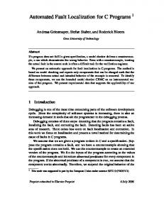
of the list l after statement i. These components are connected because they manipulate the same list. Given the input data, the network is initialized, values are propagated forward through connections to the output of the network. 3. l.insert(20)

l1 1. l=new LinkList(2)

l3

X

5. l.insert(5)

l4

l5

l2 cyclic(l2 )

4. l.insert(3) b

2. if (b) {...}

Property 1 List l is always acyclic. The code is truly simple. However we have already introduced a bug in the code. What can go wrong is that the insert(v ) does not respect Property 1; it creates a cyclic list when it is ever called on a list with a single element. Invoking the buggy insert() method on a list possibly corrupts the list. However, the corrupted list can grow further with new elements. So we have to wait even longer until the corrupted list manifests itself as observably incorrect behavior. As an example, we have written a demo(b) method in Figure 1. There is an error trace [1, 2, 3, 4, 5, 6] in the demo() method, where the corrupted list l manifests itself as an infinite loop because the size() method is going through the entire list to calculate the length. To diagnose data structure inconsistencies, we follow the MBSD framework [Mayer et al., 2002]. The program model is defined by the structure of a component network and behaviors of all components. While the structural part corresponds to syntactic entities, the behavior part implements the language semantics. Formally, a diagnosis system is a tuple (SD, COMPS , TC ), where SD is a logical description of the program model, COMPS the set of components representing statements, and TC denotes the test case describing the input data, the output data and the specification SPEC of correctness. To handle the specification of structural properties, we keep track on object relations in our program model. An object relation is a structure that relates objects; it consists of objects and their accessible objects. Given object relations, we can check user-provided structural properties and thus detect a corrupted data structure. Consider the demo(b) method, we represent it as a component network as shown in Figure 2, where each statement is mapped to a component, and connection li holds the value

Figure 2: Diagnosing error trace [1, 2, 3, 4, 5] From the execution trace [1, 2, 3, 4, 5], we observe a corrupted list l2 after statement 5 (denoted by predicate cyclic(l2 ) in Figure 2). Starting from statement 5, we go back through all statements [1, 2, 3, 4, 5], compute the witness cyclic(l ) at each statement, and thus to see where the data structure inconsistency actually originates. A contraction is raised at connection l3 , marked by X in Figure 2. This is because component l .insert(20 ) receives an acyclic list but sends a cyclic list. So we cannot assume statements 1, 2 and 3 work correctly at the same time. Thus we have three single fault diagnoses {AB (1)}, {AB (2)}, and {AB (3)}, where predicate ¬AB (i) denotes a correctly working statement i. The diagnoses pinpoint the flaw in the insert(v ) method, i.e., the list become cyclic when it is used to insert the second element. This is informative for the user, giving a hint on how the flaw could be corrected. In contrast, the VBM is less informative. An assertion l .next.next.next.next ! = l is used to specify the expected behavior of the demo(b) method. Surely this assertion is violated. The VBM’s diagnosis is that all statements 1, 2, 3, 4, 5 are possibly faulty because they influence the value of the assertion. Of course, the diagnosis is not false, but it obscures the original source of error.

3

Specification over Object Store

Structural properties are formulas defined over object relations. Since objects have types, object relations are thus typed. Definition 1 (Object Relation) An object relation R with type (T1 → ... → Tk ), denoted by R : T1 → ... → Tk , is a set of tuples (o1 , ..., ok ) such that for 1 ≤ i ≤ k, object oi is of type Ti .

Let’s call an object relation with k-tuples a k-relation. 1relations and 2-relations are said to be unary and binary. Example 1 We think of a unary relation as a table with a single column, a binary relation as a table with two columns. 1. Let x be a program variable that references an object o of type T . Then x : T is a unary relation of type T , which is a singleton set {(o)}. 2. Let A be a set of objects of type T . Then A : T is a unary object relation of type T , which is a set {(o) | o ∈ A}. 3. The next field of a LinkedList makes a binary relation next : LinkedList → LinkedList. A data structure explicitly declares various binary relations. For any field f of an object x, f is a binary relation because x.f can access at most one object. So we have: Corollary 1 Let x.f be a field access that represents an object. f is a binary relation. Set operators and relational operators provide us a means to derive new relations. The relational operators in our concern are concatenate and join 1 . Definition 2 (Concatenate Operator) 0 be two reLet p : T1 → ... → Tk and q : T10 → ... → Tm lations. The concatenate p ⊕ q of relations, with type 0 ), is a set {(p1 , ..., pk , q2 , (T1 → ... → Tk → T20 ... → Tm ..., qm ) | (p1 , ..., pk ) ∈ p, there is a tuple (q1 , ..., qm ) ∈ q, such that pk = q1 and Tk = T10 }. Definition 3 (Join Operator) 0 be two Let p : T1 → ... → Tk and q : T10 → ... → Tm relations. The join p ◦ q of relations, with type 0 (T1 → ... → Tk −1 , → T20 ... → Tm ), is a set {(p1 , ..., pk−1 , q2 , ..., qm ) | (p1 , ..., pk ) ∈ p, there is a tuple (q1 , ..., qm ) ∈ q, such that pk = q1 and Tk = T10 }. If we apply the concatenate operator and join operator on the same input relations, the join contains less columns. For example, a Tree class declares two binary relations: left : Tree → Tree and right : Tree → Tree. Whereas left ⊕ right is a 3-relation that concatenates left and right, left ◦ right is a binary relation. Moreover, let A : Tree be a unary relation holding a set of objects of type Tree, the joint A ◦ left is a set of objects accessed by the objects in A through the field left. By repeatedly applying the join operator, we can compute the transitive closure of a binary relation R, denoted by R∗ . Given binary relations, we can create new k-relations by concatenating them and joining them. Therefore, we just keep track on binary relations when modeling the input program. Putting them together, we write structural properties as formulas. For example, Property 1 is represented by: ∀x ∈ l ◦ next∗ ⇒ x ∈ / x ◦ next∗

(3.1)

which says that a list l is acyclic if there is no element in list l that can access itself. 1 Essentially they generalize the standard product and join operators.

Object relations have their origins and histories; they are like variables in that they have different values at different program points. So a relation is said to be a parent relation if it is the origin of other relations. An object relation is a child if it has a parent relation. Moreover, we introduce the term relation variable. Definition 4 (Relation Variable) A relation variable is a variable T.f , where f is a binary relation f : T → T 0 . The value assigned to a relation variable is a set of pairs in the form (i1 , i2 ) where i1 and i2 are of type T and T 0 respectively. Since we implement a set of methods to perform a consistency checking on a relation variable, the violation of structural properties is detected if we know the variable value. Definition 5 (Object Store) An Object Store is a collection of relation variables and their values.

4

Object Store Model for Debugging

In this section, we use an example to introduce the Object Store model for debugging. To do so, we first have a look at the model in Section 4.1, then we present the algorithm for compiling the program into models in Section 4.2. Finally, we explain how the model is used for debugging. Throughout this section, L is abbreviated for LinkedList.

4.1

The Model

The model in our concern is a component network as shown in Figure 3 beside the code. Let’s have a look at the dashed rectangle labeled by the statement c = this. Example 2 Components this and c = implement the semantics of statement c = this. Their connections are variables. Moreover, dark grayed components denote components that model object relations arising from variable assignments, field accesses and field assignments. • Component pt1 is said to be a relation component that holds a points-to relation pt : Var → L, which maps a set Var of variables to objects they reference to. • By default, a relation component has three input ports and one output port. For example, two of the input ports of component pt1 are used to receive the input instance from this1 and c1 . The remaining input port is used to receive the parent relation L.pt[0 ]0 , and the output port is used to send the child relation L.pt[0 ]1 . In the example, L.pt[0 ]0 andL.pt[0 ]1 describe the history of relation L.pt. Formally, we introduce indexed relation variables as follows: Definition 6 (Indexed Relation Variable) An indexed relation variable is NAME [PATH ]IDX , where NAME is a relation variable name, PATH is a sequence of numbers denoting execution branches, and IDX is an index. In the implementation, the algorithm assigns a new unique number to each branch and an index to each variable. So the PATH of a new index relation variable is the combination of its parent’s PATH and the current branch.

1. c = this; 2. p = this; 3. if (cond) { 3.1 p.next = new L(); 3.2 p = p.next; 3.3 p.next = c; }

1. c = this {} L.pt[0]0 1 this this 0

c = c01

pt1

L.pt[0]1 {(c, 0)}

p2 L.next[2]0 new L()

1

p2

0

0

next3.1 L.next[2]1 {(0, 1)}

this1 p2 0

p.next

pt2

1

if

cond

2. p = this

L.pt[0]3

L.pt[0]2 {(c, 0), (p, 0)} p = p13.2

next3.2 L.next[2]2 {(0, 1)}

p3.2

pt3.2 L.pt[2]1 {(c, 0), (p, 1)}

L.pt[2]2 L.next[2]4

c1

0

next3.3 L.next[2]3

X

{(0, 1), (1, 0)}

3.1 p.next = new L()

3.2 p = p.next

3.3 p.next = c

3. if (cond) {...}

Figure 3: An example of the Object Store Model

4.2

Model Building Process

To compile the program into models, we assume each syntactic entity has a function buildOSM which maps itself into a component, links its input ports, possibly propagate forwards static information, and returns its output connection. Statement by statement, we convert classes and methods successively and return a set of components defining the diagnosis system. The static information in our model are location pairs, denoted by pairs of numbers that abstract the run-time objects and approximate the semantics of four syntactic entities: class creation, object variable assignment, field access and field assignment. Similar to [Mayer et al., 2002], the algorithm maps loops and method calls to hierarchic components with inner submodels. For example, the loop component contains two submodels: MC and MB , where MC denotes the sub-model of the loop condition, and MB the sub-model of the loop body (represented as a nested if-statement 2 ). For each class the inherited methods are compiled into models. At debugging time, the actual class of the invoked method is available and therefore the correct method call will be used. We further assume that env represents the working environment of components, connections, and the indices assigned to variables. The algorithm is summarized in Figure 4, where c denotes a component and the following auxiliary functions are used: • Function addComp(env , c) adds a component c into the environment env . • in(c) denotes the input connections of c. • out(c) denotes the output connections of c. • Function propagate(c) receives the static information from the input ports of a component c, stores the input instance, unifies it with the value of the parent relation, and propagates them to the output port of c. • Function conn : (ENV , EXP ∪ Var ) 7→ CONNS maps expressions or variables to connections by using an environment. • Function parent : (ENV , EXP ) 7→ CONNS looks up in the environment for a set of parent relations named by the input expression3 . If none, a parent relation is created. • Function modifiedConn(env ) returns a set of connections denoting variables with new values. 2

The nesting size is obtained by computing all pairs shortest path in a dependency graph (see [Wieland, 2001])

• path(env ) is a number denoting the current branch. • newComp(type, exp, env ) is a function that returns a new component of type, which is initialized by the following steps: 1: c = new Ctype 2: addComp(env , c) 3: out(c) = conn(env , exp) 4: in(c) = buildOSM (exp, env ) 5: return c • newRelation(c, vp , type, env ) is a function that returns a new relation component of type, which is initialized by the following steps: 1: c0 = new Ctype 2: addComp(env , c 0 ) 3: out(c 0 ) = conn(env , vp ) 4: in(c 0 ) = {vp } ∪ out(c) ∪ in(c) 5: return c0 Example 3 Consider the code in Figure 3, which is taken from the insert(v ) method in Figure 1 and represents the case that the loop body of the while-statement is not executed. In the model as shown in Figure 3, we neglect some components that provide inputs for relation components. However, the inputs from the missing components are labeled by variable vi , which denotes that program variable v gets the value on the statement i. Now let’s go through statements 1 ∼ 3 to see what is going on behind the picture in Figure 3. • 1. c = this; The algorithm first creates an assignment component c =. Then it maps this to component this, as the input to component c =. Since this is used, location 0 is created to approximate the run-time object referenced by this. So the output connection c1 has the value 0. Finally the algorithm handles the object relation arising from this statement. Since parent(env , c) fails to find a parent relation pt : Var → L and path(env ) = 0, a new indexed relation variable L.pt[0]0 is created in the environment and initialized as empty. With newRelation(c =, L.pt[0], pointstoRelation, env ), relation component pt1 is thus created and receives inputs from this1 , c1 , and L.pt[0]0 . Therefore {(c, 0)} is stored in pt1 and propagated to its output connection L.pt[0]1 . 3 For an object variable w, the name is T.pt, where T is w’s class type. For a field access v.f , the name is in the form of T.f where T is w’s class type

buildOSM (v = new C, env) c = newComp(assignment, new C, env) for all vp ∈ parent(env, v) c0 = newRelation(c, pointstoRelation, vp , env) propagate(c0 ) endfor buildOSM (v = w, env) c = newComp(assignment, w, env) for all vp ∈ parent(env, v) c0 = newRelation(c, pointstoRelation, vp , env) propagate(c0 ) endfor buildOSM (v.f, env) c = new Cf ieldaccess addComp(env, c) in(c) = conn(env, v) out(c) = conn(env, v.f ) for all vp ∈ parent(env, v) c0 = newRelation(c, vp , objectRelation, env) propagate(c0 ) endfor buildOSM (v.f = w, env) c = newComp(f ieldassignment, w, env) for all vp ∈ parent(env, v) c0 = newRelation(c, objectRelation, vp , env) propagate(c0 ) endfor buildOSM (if (Exp) then S1 else S2 , env) c = new Cif addComp(env , c) cond = buildOSM (Exp, env ) oldpath = path(env ) path(env ) = path(env ) + 1 Let env 0 be a copy of env buildOSM (S2 , env 0 ) path(env ) = path(env ) + 1 Let env 00 be a copy of env buildOSM (S1 , env 00 ) create an input port of c and connect it to cond Let A = modifiedConn(env 0 ) ∪ modifiedConn(env 00 ) for all x ∈ A if x ∈ modifiedConn(env 0 ) create an input port of c and connect it to x endif if x ∈ modifiedConn(env 00 ) create an input port of c and connect it to x endif create an output port of c and connect it to a new connection x0 named by x remove x from modifiedConn(env ) add x0 into modifiedConn(env ) endfor path(env ) = oldpath Figure 4: Algorithm for converting Java code

• 2. p = this; Similar to statement 1, component pt2 is created and gets the input instance {(p, 0)}. Then pt2 propagates the union of input instances to its output connection L.pt[0]2 . • 3. if (cond ){...}; The algorithm first maps the if-statement to a component if and converts the condition cond . Then it stores its current path(env ) and converts the else-branch by using a new environment env 0 with path(env 0 ) = 1. We convert the then-branch with a new environment env 00 and path(env 00 ) = 2 as follows: – 3.1 p.next = new L(); First p.next is mapped to a new field assignment component (neglected in Figure 3). Next new L() is mapped to a class creation component, which contains sub-models of class constructors. To model the newly-created object, a fresh location 1 is used and put on the output connection of component new L(). Relation component next 3.1 is then created to handle the object relation. It receives inputs from p2 , component new L() and a new indexed relation variable L.next[2]0 (created and initialized because parent(env , c) fails to find a parent relation next : L → L and path(env ) = 2). Finally input instance {(0, 1)} is stored in next 3.1 and propagated to its output connection L.next[2]1 . – 3.2 p = p.next; It creates components next 3.2 and pt 3.2 . Then next 3.2 receives values from p2 , L.next[2]1 , and component p.next. So the input instance {(0, 1)} is stored in next 3.2 and we have L.next[2]2 = {(0, 1)}. When pt 3.2 receives values from p3.2 , L.pt[0]2 , and component p.next, the input instance {(p, 1)} is stored in pt 3.2 and we have L.pt[2]1 = {(c, 0), (p, 1)}. – 3.3 p.next = c; It creates component next3 .3 which receives values from p3.2 , c1 , and L.next[2]2 . So the input instance {(1, 0)} is stored in next 3.3 . Unifying with the value of L.next[2]2 , we have L.next[2]3 = {(0, 1), (1, 0)}. • After both branches are converted, component if takes all inputs from variables in the two branches where they have new values, and creates new connections to be used in subsequent statements.

4.3

Diagnosing with the Model

Given the test case, input and output values are propagated forward and backward throughout the network. A contradiction is raised in the diagnosis system when (1) a variable gets two or more different values from different components, or (2) a relation variable violates a certain property but its parent does not. A conflict is defined by a set of components causing the contradictions. To diagnose Property 1, we run the model in Figure 3 by assuming cond is true. As revealed by the solid line, the runtime object relations are propagated forward from the input to the output. In the forward propagation, locations are binded with run-time objects at each relation component. For example, location 0 (1) is binded with object o0 (o1 ) at component next 3.1 . So we have a contradiction at connection L.next[2]3

= {(o0 , o1 ), (o1 , o0 ), . . . } because it is a cyclic list but its parent is not. This misbehavior is explained by assuming that components if and next 3.3 behave incorrectly.

5

First Results

To evaluate the Object Store model, several example programs have been created. The example programs implement a shape class and various data structures such as linked list, stack, tree, etc. (see Table 1), where the OA column shows the number of object accesses. All programs involve various control flows, virtual method invocation, and object-oriented language notations, such as multiple objects, class creations, instance method calls, class and instance variables, etc. Program LinkedList

Main Methods

Lines [#] 58

OA [#] 20

insert, remove, join, reverse Stack push, pop, etc. 67 22 Shape overlap,scaleBy, 200 120 transpose, rotate ExpressionTree insert,remove, 146 58 left, right, etc. Table 1: Benchmarks and debugged methods The diagnosis experiments are performed on example programs with a seeded fault. The results are summarized in Table 2, where it depicts the elapse time for modeling (M-G column), the elapsed time for computing diagnoses (T-D column), and the number of diagnosis (N-D column). The right column lists the result obtained by diagnosing with a VBM. Compared with the VBM, it is shown that the number of diagnosis candidates is reduced and all diagnosis candidates are in the VBM’s diagnosis. So our model hits the original source of error sufficiently and accurately, directing attention to the root cause of a property violation. Finner diagnosis is achieved by descending into the faulty method calls or blocks of statements. Program

M-G T-D N-D VBM [sec.] [sec.] [#] N-D LinkedList 0.6 0.3 3 10 Stack 0.6 0.4 1 4 0.9 0.4 2 4 Shape 2.3 0.3 1 5 ExpressionTree 7.2 2.5 4 9 Table 2: Comparison of empirical results Currently we are not working on programs with exceptions, threads and recursive method calls. The Archie system [Demsky and Rinard, 2003] is close to our work. But there is no guarantee that the original source of all data structure corruption errors are captured in Archie because the consistency checker is invoked periodically.

6

Conclusion

In this paper, we present an Object Store model to diagnose data structure inconsistencies. Our approach hits both the structural properties and their implications by reasoning about object relations arising from the program execution. We have used the approach to isolate errors in several small Java programs to prove their principal applicability. The maximum time complexity of the buildOSM algorithm is of order o(2 |N | ), where N is the number of branch

nodes in the control flow graph (CFG) of a method of the input program. This worst time complexity is acceptable because the CFG of a method is usually very small. The worst time complexity of diagnosing a property P is of order o(T (Π ) + size(Π ) · T (P )), where T (Π ) is the maximum time for computing error trace Π and T (P ) the maximum time of checking property P . The optimization of inconsistency detection helps us scale the Object Store model to middle-sized problems. This is because the overall costs of detecting inconsistency can be reduced if the structural properties are checked against objects binded with locations. To help the developer to understand the essence of the program error, we are beginning to generate an error explanation on the basis of fault locations and the counterexample of a structural property. It is revealed in Figure 3 that static information is an abstraction of program behavior; for example, L.next[2]3 = {(0, 1), (1, 0)} indicates at compile-time that a cyclic list is created. So further research will explore how static analysis can assist us to rank user-provided properties.

References [Ball et al., 2003] T. Ball, M. Naik, and S.K. Rajamani. From symptom to cause: localizing errors in counterexample traces. In Proc. of POPL, pages 97–105. ACM Press, 2003. [Bush et al., 2000] William R. Bush, Jonathan D. Pincus, and David J. Sielaff. A static analyzer for finding dynamic programming errors. Software Practice and Experience, 30(7):775–802, 2000. [Clarke et al., 2000] E. Clarke, O. Grumberg, and D. Peled. Model Checking. The MIT Press, Cambridge, Massachusetts, 2000. [Demsky and Rinard, 2003] Brian Demsky and Martin Rinard. Automatic detection and repair of errors in data structures. ACM SIGPLAN Notices, 38(11):78–95, 2003. [Detlefs et al., 1998] David L. Detlefs, K. Rustan M. Leino, Greg Nelson, and James B. Saxe. Extended static checking. Technical Report SRC-RR-159, HP Laboratories, 1998. [Groce, 2004] A. Groce. Error explanation with distance metrics. In TACAS, volume 2988 of Lecture Notes in Computer Science. Springer, 2004. [Jackson, 1995] Daniel Jackson. Aspect: Detecting Bugs with Abstract Dependences. ACM TOSEM, 4(2):109–145, 1995. [Mayer et al., 2002] W. Mayer, M. Stumptner, D. Wieland, and F. Wotawa. Can ai help to improve debugging substantially? debugging experiences with value-based models. In Proc. ECAI, pages 417–421. IOS Press, 2002. [Reiter, 1987] Raymond Reiter. A theory of diagnosis from first principles. Artificial Intelligence, 32(1):57–95, 1987. [Wieland, 2001] D. Wieland. Model-Based Debugging of Java Programs Using Dependencies. PhD thesis, Vienna University of Technology, Institute of Information Systems (184), Nov. 2001. [Zeller and Hildebrandt, 2002] Andreas Zeller and Ralf Hildebrandt. Simplifying and isolating failure-inducing input. IEEE Transactions on Software Engineering, 28(2), 2002.