AUTOMATIC AND ROBUST FOREARM SEGMENTATION ... - CiteSeerX

AUTOMATIC AND ROBUST FOREARM SEGMENTATION USING GRAPH CUTS P. F¨urnstahl1 , T. Fuchs2, A. Schweizer3 , L. Nagy3 , G. Sz´ekely1 , M. Harders1 1

Computer Vision Laboratory, ETH Zurich, Zurich, Switzerland Institute of Computational Science, ETH Zurich, Zurich, Switzerland 3 Department of Orthopedic Surgery, University Hospital Balgrist, Zurich, Switzerland 2

ABSTRACT The segmentation of bones in computed tomography (CT) images is an important step for the simulation of forearm bone motion, since it allows to include patient specific anatomy in a kinematic model. While the identification of the bone diaphysis is straightforward, the segmentation of bone joints with weak, thin, and diffusive boundaries is still a challenge. We propose a graph cut segmentation approach that is particularly suited to robustly segment joints in 3-d CT images. We incorporate knowledge about intensity, bone shape and local structures into a novel energy function. Our presented framework performs a simultaneous segmentation of both forearm bones without any user interaction. Index Terms— forearm, segmentation, bone, graph cut 1. INTRODUCTION Treatment goals in the care of forearm fractures are bone healing and restoration of function. Bone union of the forearm shaft in an incorrect anatomic position impairs the rotation of the forearm (i.e. pronation and supination). This may result in reduced range of motion, pain, and instability during forearm rotation. For individual planning of a corrective osteotomy a method to obtain the shape of the bone is needed, in order to simulate the pathological forearm kinematics. Therefore, an accurate and robust segmentation of both forearm bones (radius and ulna) in 3-d computed tomography (CT) datasets is required. In general, long bone segmentation is a straightforward task since cortical bone, which is dense and compact, forms the bone surface. Due to its high density a bone shaft appears very bright in a CT image. The spongy interior layer, the cancellous bone, is much less dense. Joints have to be more flexible and therefore they mainly consist of cancellous bone. Thus, contrast between joints and the surrounding tissue in an image is much less pronounced. This is in particular the case for elderly patients whose bone density is decreased. In addition to weak joint boundaries, the articular spaces between radius, ulna and carpal bones are extremely narrow. This results in diffuse boundaries between the joint components that This work has been supported by the Swiss National Science Foundation

appear as being in direct contact in the CT image due to partial volume effects. Since the forearm joints have a crucial influence on the kinematics, an algorithm is required that can accurately segment the bone joints under these conditions. We therefore propose a framework that performs an automatic segmentation of both forearm bones, using graph cut optimization. Particular attention is paid to the segmentation of the distal and proximal radio-ulnar articulation which is a challenging task. As a key contribution we introduce novel energy functions for segmentation of sheet-like objects with weak boundaries. We also tackle the problem of differentiating objects with extremely small inter-object spacing. Several methods have been proposed to segment bones and joints from CT images. Sebastian et al. [1] use a skeletally coupled deformable model for the segmentation of carpal joints. The problems of joint segmentation are discussed in detail. An excellent overview and comparison of well-known segmentation methods like tresholding, region growing, region competition, watershed, and deformable models is also given. Westin et al. [2] and Descoteaux et al. [3] use local structure tensors for bone enhancement. Our paper also incorporates this measure in the segmentation algorithm. Neubauer et al. [4] use thresholding, followed by a manually initialized watershed algorithm to segment radius, ulna, and carpus for a virtual corrective osteotomy application. Hahn [5] also proposes an interactive watershed transform for bone segmentation. In both approaches user-interaction is necessary for a successful segmentation. A growing number of image segmentation approaches use energy minimization techniques. Snel et al. propose a 3-d active contour model for the detection of carpal bones [6]. The segmentation result depends on the quality of an initial contour, which is hard to obtain automatically. Level sets and graph cuts are global optimization techniques to minimize energy functions. A 3-d active contour approach using level sets for the segmentation of anatomical structures was proposed by Zushkevich et al. [7]. Boykov and Jolly [8] introduced a technique that uses graph cuts for interactive segmentation of N -dimensional images. This basic strategy was extended subsequently by different groups. An excellent overview of recently published approaches is given by Boykov and Funka-Lea [9].

2. METHODOLOGY

2.1.1. Graph cut background

The key idea of the segmentation framework is that the algorithm identifies the radius and the ulna in a slice by slice fashion in axial direction, starting from an initial slice. This allows for incorporating prior-knowledge, gained from previously segmented slices, into the segmentation process. A positive side-effect is that the area, where the graph cut has to be applied, can be narrowed down to a smaller image patch since the extent of each bone in the previously segmented slice is known. At first, the start slice has to be chosen and an initial labeling of the bones of interest in it has to be provided since no prior knowledge is available. The center slice of the dataset is a good choice as a starting point because the bone density is strongest in the middle part of the bones. For this, it is assumed that the imaged anatomy corresponds to the forearm. The initial segmentation of radius and ulna is achieved by thresholding (threshold of 400 HU), followed by a connected component labeling algorithm, where the two largest components are choosen. Starting from the center slice, radius and ulna are simultaneously segmented by applying the slice-wise segmentation, described in Section 2.1, in both z-directions. The segmentation of a bone is terminated, when the number of segmented voxels for this component falls below a certain threshold (i.e. 20 voxels) in the currently processed slice.

2.1. Slice-wise segmentation At first the image patches, where the actual segmentation is applied, are determined for the current slice. To this end the bounding rectangles of radius and ulna are calculated based on the segmentation result of the previous slice. The new patches are obtained by enlarging each bounding rectangle by a factor δ, which must be large enough to cover the size change of the bone between two slices. We set δ to two times the slice-spacing. In each patch P the encompassed bone has to be segmented, that is we want to find the optimal labeling l that assigns a voxel v ∈ P either label ”object” or ”background” and minimizes the standard energy function [10] E(f ) =

X v∈P

Dv (lv ) +

X

Vv,w (lv , lw ),

(1)

v,w∈N:lv 6=lw

where N is the set of pairs of adjacent voxel. Dv (lv ) is the data cost function that measures the costs for assigning voxel v to label lv . Vv,w (lv , lw ) measures the costs for assigning voxel v to label lv and neighbor w to lw (smoothness costs). Polynomial time algorithms exist which minimize Equation 1 by calculating a minimum cut across a graph [10, 11]. In the following sections we describe how the graph is constructed and introduce appropriate data and smoothness cost functions that are used to segment the bones.

A graph G(V, E) of an image is constructed by associating the image voxels to the nodes of V and connecting neighboring voxels with edges contained in E. In this graph-based segmentation approach two additional nodes are contained in V called terminals. The terminals correspond to labels which can be assigned to voxels. In order to assign a certain label to voxels, not only edges between two voxels (n-links) are included in E, but also edges which connect the voxels to the two terminals (t-links). The weight of a t-link, connecting a voxel v and a terminal, indicate the costs for assigning the voxel to this label. n-link weights represent spatial relation between neighboring voxel. In terms of energy minimization, weights assigned to t-links and n-links reflect the parameters in the data cost and smoothness cost terms of the energy function in Equation 1. The minimum cost cut then represents a labeling which optimizes this energy function. 2.1.2. Data cost function Typically intensity distributions, often based on manually positioned seeds, are used to set up the data costs for the remaining voxels. This is hardly possible in our case, since the intensities of both bone and soft tissue vary significantly dependent on their position. Therefore, we have developed an accurate estimation of the intensity values of bone and tissue which also encodes spatial information. Intensity changes between two slices are relatively small in a local neighborhood, since the shape of radius and ulna varies slowly in axial direction. Based on this observation, a 2-d intensity map Ψb is generated in order to predict the bone intensities on the next slice. To this end, a mean intensity is calculated for each bone-labeled voxel of the previously segmented slice by averaging the intensity value of each bonelabeled voxel in a certain neighborhood (i.e. 5 × 5). The mean values are stored in a map according to the 2-d positions of the corresponding voxels. A modified distance transform is then applied to the map. Instead of storing a distance at each map position, the mean intensity of the nearest bone-labeled voxel is stored. In the same manner an intensity map Ψt for soft tissue, which surrounds the segmented bone, is generated. Using the proposed intensity maps, intensity estimates of the nearest bone- or tissue-labeled voxel can be extracted in constant time. A labeling only based on intensity maps is unstable when intensity differences between soft tissue and bone are too small to make a clear differentiation. In order to gain more robustness, the intensity measure is combined with a sheetness measure that enhances bone structures [3]. The sheetness of a voxel v is defined as

(

S(v) =

0 (exp

λ3 > 0, if−R  2 s

2α2

)(1 − exp

 −R2 

 −R2 

2β 2

2c2

b

)(1 − exp

n

)

,

where α, β, and c are set respectively to 0.5, 0.5 and half the maximum Frobenius norm of the Hessian matrix [3]. The ratios Rs = |λ2 |/|λ3 |, Rb = |(2|λ3 | − |λ2 | − |λ1 |)|/|λ3 |,

p Rn = λ21 + λ22 + λ23 are defined by the eigenvalues λ1 ,λ2 , and λ3 (sorted in ascending order) of the Hessian matrix at v. Finally, the total data costs for a voxel v with intensity Iv are

8 β < |Iv −Ψσ b (v)| (1 − S(v))1−β , if f = bone  Dv (f ) =  , : |Iv −Ψt (v)| β S(v)1−β , if f = tissue σ where Ψb (v) and Ψt (v) are the intensity maps for bone and tissue. S(v) is the normalized sheetness function and σ is a normalization factor for the intensity term which was set to |Ψb (v) − Ψt (v)|. A β-value of 0.8 was used in all experiments. 2.1.3. Smoothness cost function Smoothness cost are used to define spatial coherence which is done by penalizing discontinuities between adjacent voxels. A cost function only based on intensity differences caused leakage in our experiments due to the presence of fuzzy edges. We therefore propose to incorporate the sheetness of neighboring voxels in the smoothness function. For two adjacent voxels v and w, where v is labeled as bone and w as tissue (lv 6= lw ), |S(v) − S(w)| is typically high at the bone boundary. In order to favor cuts near the boundary, the smoothness cost has to be small if |S(v) − S(w)| is high. Additionally, the shape of the bone is incorporated into the smoothness term. As proposed in [12], we use a shape prior based on a level-set template. The boundary of the segmented bone of the previous slice defines this template. Let Φ(v) be a function that returns the distance of v to the template boundary. Then Φ((v + w)/2) is small when both voxels v, w lie near the template boundary, as desired. Combining both measures, the smoothness costs for voxels v and w are defined as Vv,w (lv , lw ) = α (1.0 − |S(v) − S(w)|)β Φ

 v + w 1−β 2

, (2)

where both functions S(v) and Φ(v) are normalized. α and β were set to 0.75 and 0.5 in all our experiments. 2.1.4. Direct contact The articular space between radius and ulna is extremely narrow which appears as direct contact in the CT images (see Figure 3). It would require a strong increase of the smoothness cost in order to prevent leakage in this area. On the other hand, this leads to incorrect segmentation results at weak, thin boundaries. Our graph cut algorithm is therefore applied without stronger boundary constraints. Potential leakage between radius and ulna is corrected in a separate step using an alternative data cost function. All voxels that are labeled as object in one image patch but actually belong to the bone in the other image patch should be labeled as background (and vice versa). Therefore a criterion has to be found which measures whether a voxel belongs to the radius or the ulna. Intensity differences in the contact area of the two bones were not significant enough in our datasets. A better measure was to compare the distances of a voxel to

the boundaries of radius and ulna in the previous slice. We achieved best results by using the mean distance Φ(v) to the boundary in an 8-neighborhood around voxel v. The new data cost function only considers voxels which are in the intersection v ∈ Pr ∩ Pu of the two image patches of radius and ulna, the labeling of remaining voxels is not modified and used as hard constraints. The data cost function for Pr and respectively Pu is defined as follows

(

Dv (f ) =

Φr (v) , if f = bone , Φu (v) , if f = tissue

where Φr and Φu are the mean distances to the boundaries of radius and ulna. After setting the data and smoothness costs (now using Equation 2 with α = 0.25, β = 0.0) the graph cuts are updated in both image patches yielding the final segmentation of radius and ulna.

Fig. 1. Surface models of segmented radius and ulna.

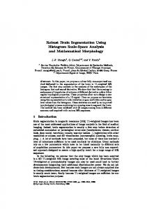
3. RESULTS In order to evaluate the proposed algorithm, we tested it on cadaver forearms in different pro- and supination positions, overall on 19 CT datasets. The inter-bone distance varies during forearm movement and therefore the algorithm must be capable of segmenting forearms in different poses. A commercial CT scanner (Philips Brilliance 40) was used for data acquisition. The in-plane resolution of all datasets was 0.29 × 0.29 mm (512×512 pixel). The number of slices ranged from 803 to 874, with a slice-thikness/slice-spacing of 0.67/0.33 mm. For all scans, the forearms were aligned with their longitudinal axis parallel to the scanner’s z-axis. Radius and ulna were successfully segmented without any user interaction in all experiments. Figure 1 shows a 3-d result of the segmented forearm bones. The algorithm processes 8 slices per second (Pentium 4, 3.2 GHz), resulting in an average runtime of 103 ± 5.4 s (24 s graph cut, 60 s sheetness measure, 19 s distance- and intensity maps). In order to evaluate the accuracy of the segmentation, we compared the outer bone boundaries with results of a manual segmentation. The average mean distance error was 0.22 mm, and the average of the maximum distance in the 19 datasets was 1.9 mm. We also compared our algorithm with three other techniques in order to show its strengths: a 3-d active contour method using level sets [7], an interactive watershed transform [5], and a standard graph cut approach with intensity based energy functions [8]. Figure 2 shows that our algorithm is clearly superior in detecting weak bone boundaries. Another benefit

is that our method is capable of segmenting the radio-ulnar joints without leakage. The tested watershed algorithm was also able to segment bones with fuzzy edges without leakage (by manually setting markers). However, neither the active contour method nor the standard graph cut approach (penalizing intensity differences) was able to individually segment the bones without leakage in any dataset (see Figure 3). 4. CONCLUSION AND FUTURE WORK We have presented a fully automatic segmentation framework for the forearm bones radius and ulna. The main contribution is the introduction of appropriate energy functions that are particularly suited for joint segmentation with weak or fuzzy edges. Additionally, the proposed smoothness term of the energy functions allows a segmentation of joints with narrow inter-bone spacing. The energy functions are minimized using a graph cut approach yielding an optimal solution. Currently, the algorithm requires CT datasets with thin and dense slices since the articular spaces between both forearm bones and the carpal bone is extremely narrow. The extension of the method, capable to handle axial resolutions up to 1 mm, is planned as future work.

(a)

(b)

(c)

(a)

(b)

(c)

(d)

Fig. 3. Joints with narrow inter-bone spacing. The resulting outer bone boundary is shown in white. (a) unsegmented patch, (b) active contour segmentation, (c) graph cut penalizing intensity differences, (d) our approach. [3] M. Descoteaux, M. Audette, K. Chinzei, and K. Siddiqi, “Bone enhancement filtering: Application to sinus bone segmentation and simulation of pituitary gland surgery,” Computer Aided Surgery, vol. 11, pp. 247–255, 2006. [4] A. Neubauer, S. Wolfsberger, M. T. Forster, L. Mroz, R. Wegenkittl, and K. B¨uhler, “Virtual corrective osteotomy,” in Computer Assisted Radiology and Surgery, 2005, vol. 1281, pp. 684–489. [5] H. K. Hahn, Morphological Volumetry : Theory, Concepts, and Application to Quantitative Medical Imaging, Ph.D. thesis, University of Bremen, 2005. [6] J. G. Snel, H. W. Venema, and C. A. Grimbergen, “Deformable triangular surfaces using fast 1-d radial lagrangian dynamics-segmentation of 3-D MR and CT images of the wrist,” IEEE Trans Medical Imaging, vol. 21, pp. 888–903, 2002. [7] P. A. Yushkevich, J. Piven, H. C. Hazlett, R. G. Smith, S. Ho, J. C. Gee, and G. Gerig, “User-guided 3D active contour segmentation of anatomical structures: significantly improved efficiency and reliability.,” Neuroimage, vol. 31, pp. 1116–1128, 2006.

(d)

(e)

Fig. 2. Segmentation of the radio-ulnar joint with weak boundary. The identified outer bone contour is shown in white. (a) unsegmented patch, (b) watershed segmentation (manual thresholding of the original data masked by the watershed basin), (c) active contour segmentation, (d) graph cut using histogram-based probability, (e) our approach. 5. REFERENCES

[8] Y. Boykov and M. P. Jolly, “Interactive graph cuts for optimal boundary & region segmentation of objects in N-D images,” in ICCV, 2001, vol. 1, pp. 105–112. [9] Y. Boykov and G. Funka-Lea, “Graph cuts and efficient N-D image segmentation,” Int. J. Comput. Vision, vol. 70, pp. 109–131, 2006. [10] V. Kolmogorov and R. Zabih, “What energy functions can be minimized via graph cuts?,” IEEE PAMI, vol. 26, pp. 147–159, 2004.

[1] T. B. Sebastian, H. Tek, J. J. Crisco, S. W. Wolfe, and B. B. Kimia, “Segmentation of carpal bones from 3d CT images using skeletally coupled deformable models,” in MICCAI. 1998, pp. 1184–1194, Springer.

[11] Y. Boykov and V. Kolmogorov, “An experimental comparison of min-cut/max-flow algorithms for energy minimization in vision.,” IEEE PAMI, vol. 26, pp. 1124– 1137, 2004.

[2] C. F. Westin, S. K. Warfield, A. Bhalerao, L. Mui, J. A. Richolt, and R. Kikinis, “Tensor controlled local structure enhancement of CT images for bone segmentation,” in MICCAI. 1998, pp. 1205–1212, Springer.

[12] D. Freedman and T. Zhang, “Interactive graph cut based segmentation with shape priors,” in CVPR, 2005, vol. 1, pp. 755–762.