Automatic Multi-organ Segmentation Using Learning ... - CiteSeerX

Automatic Multi-organ Segmentation Using Learning-Based Segmentation and Level Set Optimization Timo Kohlberger1, Michal Sofka1 , Jingdan Zhang1 , Neil Birkbeck1 , Jens Wetzl1 , Jens Kaftan2 , J´erˆome Declerck2 , and S. Kevin Zhou1 1

Image Analytics and Informatics, Siemens Corporate Research, Princeton, NJ, USA 2 Molecular Imaging, Siemens Healthcare, Oxford, UK

Abstract. We present a novel generic segmentation system for the fully automatic multi-organ segmentation from CT medical images. Thereby we combine the advantages of learning-based approaches on point cloudbased shape representation, such a speed, robustness, point correspondences, with those of PDE-optimization-based level set approaches, such as high accuracy and the straightforward prevention of segment overlaps. In a benchmark on 10–100 annotated datasets for the liver, the lungs, and the kidneys we show that the proposed system yields segmentation accuracies of 1.17–2.89mm average surface errors. Thereby the level set segmentation (which is initialized by the learning-based segmentations) contributes with an 20%-40% increase in accuracy.

1

Introduction

Discriminative segmentation approaches have proven to give reliable, fully-automatic, and fast detections of anatomical landmarks within volumetric images, as well as the accurate determination of organ boundaries, such as of the inner and outer walls of the heart, [10], or of the liver, [4]. Usually, the segmenting surface is represented by relatively low number of explicit control points, such as they are used in Active Shape Models. Besides restrictions in topology, other well-known disadvantages of point cloud-based shape representations are the dependence of the local detailedness on the local density of control points. The latter often are non-homogeneously distributed across the shape boundary, and thus yield varying levels of segmentation accuracy. Level set-based shape representations, see [1] and the references therein, on the other hand, provide a well-known mean to encode segment boundaries at a homogeneous resolution, with simple up- and down-sample schemes. Moreover, in the case of multiple objects, the detection and formulation of constraints to prevent overlaps between adjacent segment boundaries can be achieved much simpler by a level set representation where signed distance functions are employed. In the following we will present a fully automatic segmentation system for multiple organs on CT data, that combines the advantages of both segmentation G. Fichtinger, A. Martel, and T. Peters (Eds.): MICCAI 2011, Part III, LNCS 6893, pp. 338–345, 2011. c Springer-Verlag Berlin Heidelberg 2011 

Automatic Multi-organ Segmentation

339

approaches and their employed shape representations in an optimal manner. In particular the point-to-point correspondences, which are estimated during the learning-based segmentation, will be preserved in the level set segmentation. With regards to the latter, we will present novel terms which allow to impose region-specific geometric constraints between adjacent boundaries. In Section 2 we first give an outline of the learning-based detection and segmentation stages, all of which have been published in the mentioned citations. After a brief description on the conversion of their output meshes to implicit level set maps, we start to build an energy-based minimization approach for multiple organs as a segmentation refinement stage. In the experimental Section 3, we first show the impact of the new constraints at qualitative examples, and finally evaluate the overall improvement of the level set refinement stage over the detection-based results at 10–100 annotated cases for the liver, lungs and kidneys.

2 2.1

Approach Anatomical Landmark Detection and Learning-Based Segmentation of Organ Boundaries

We initialize the multi-region level set segmentation from explicitly represented boundary surfaces stemming from an existing learning-based detection framework, which itself consists of several stages. In the first stage, a landmark detection system estimates key organ landmarks ranging from the abdominal to upper body region, see [5] for more details. These landmarks then serve a initializations for a hierarchical bounding box detection system based on Marginal Space Learning [10] in connection with Probabilistic Boosting Trees [9]. The latter yields bounding box estimates for the liver, the left and right lung, the heart, and the kidneys. In the third stage, organ-specific boundary detectors are employed to evolve the correct organ boundaries on a coarse scale and in subsequently on a fine scale, see [4]. In addition, PCA-based statistical shape model are used to regularize the boundary shape on the coarse resolution. Thereby, segment boundaries of each organ are represented by a triangulated mesh, i.e. a connected point-cloud as being used in Active Shape Models. 2.2

From Meshes to Zero-Crossings of Signed Distance Maps

Although the learning-based segmentation sub-system already provides good individual organ segmentations, see Fig 2(a) for example, they usually exhibit small overlaps between adjacent organ boundaries, or gaps where the true organ boundaries coincide. Given representations of only the adjacent segments’ boundaries, those deficiencies are difficult to detect and remove. Instead we initialize signed distance functions φi : R3 ⇒ R from each of the result meshes Ci , for i, . . . , N organs by employing a fast mesh voxelization algorithm. The boundary information then is encoded implicitly in the zero-crossings of the φi , i.e.

340

T. Kohlberger et al.

Ci := {x | φi (x) = 0, |∇φ| = 1}, with |∇φ| = 1 denoting the so-called distanceproperty, and φ > 0 inside the object and < 0 outside, see [1] and the references therein. The distance functions are discretized on a regular grid, which, in the following, is assumed to be the same for all organs. Furthermore, we employ a narrow-banded level set scheme, which maintains the distance-property in a small narrow-band of ±2 voxels from the zero crossing. In addition to the distance functions, we still keep the mesh points, denoted by {pi }, and are tracking them along with the evolving zero crossing as described in [3], since they provide point-wise correspondences to the mean shape of the PCA model employed in the preceding learned-based boundary detection step. 2.3

Data and Smoothness Term of the Level Set Approach

Having the triangulated boundary meshes {Ci } of the detection stages transfered to distance functions functions {φi }, detecting and removing local overlaps and gaps between them can be realized much easier. The ultimate target of course is to find the correct separating boundary between two neighboring organs. To that end, in the following, we propose a level set segmentation approach which not only refines the segmentation boundary accuracy, removes local overlaps and gaps, but also finds the true separating boundary given that enough image information is available. For each organ Oi , this refining level set segmentation is realized by employing gradient descent iteration to converge to a minimum of an associated energy functional Ei (φi ), given the initial distance maps as starting points, see [1] and the references therein. As data-dependent energy term, we here employ    Ep (φ) = −α H(φ) log pin (I(x)|φ) + 1 − H(φ) log pout (I(x)|φ) dx , Ω

with H denoting the Heaviside step function, and pin/out referring to nonparametric probability estimates of the intensities inside and outside, respectively, of the current segment φ using a Parzen density estimator with a Gaussian kernel, see [2] for further details, and α being a constant weight. In order to add robustness against noisy data, we furthermore incorporate the boundary smoothness regularization term  Ec (φ) = γl(x) |∇H(φ)| dx, with l(x) = arg min x − pi L2 , (1) Ω

i=1,...,N

which employs a weight γl(x) that varies with the location on the boundary. The latter is realized by assigning fixed weights {γi } to each of the correspondence points {pi } on the mean shape of the PCA shape model, which then are tracked along during the zero-crossing evolution, see [3] for more details. 2.4

Disjoint Constraint to Remove Overlaps

0 0 Let CA and CB be detected boundaries of the learning-based stage in the case of 0 0 two adjacent organs A and B, and assume that CA and CB imperfectly overlap

Automatic Multi-organ Segmentation

341

each other to a certain degree, see, e.g., Fig. 1(a). By representing these two ˜ inside the oversurfaces using signed distance functions φ0A and φ0B , locations x lapping region are exclusively characterized by φA (˜ x) > 0 and φB (˜ x) > 0, and thus provide a much simpler overlap indicator compared to any other based on an explicit shape representation. Subsequently, additional energy terms which explicitly penalize overlaps usually are of the form      Eo (φA , φB ) := H φA (x) H φB (˜ x) φB (˜ x) dx (2) Ω

where the first product in the integrand is unequal zero only inside the overlap regions, see Fig. 1(b). In addition to similar terms such as proposed in [6], we propose to also multiply with the second distance function φB which makes EO smoother at the presence of small overlaps, and thereby decreases oscillations during gradient descent. The corresponding energy gradient reads (cf. [7]):   ∂φA /∂t = −∂Eo /∂φA = −δ (φA ) H φB (˜ x) φB (˜ x) . (3)

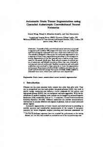
Fig. 1. Imposing geometric constraints to remove overlaps (b) and gaps (c) from an existing segmentation, while controlling the deviation from a given shape locally (d). (Note that (b)–(d) are 1D-cuts along the black lines in (a)).

2.5

Local Proximity Constraint to Fill Gaps

With regards to removing erroneous gaps between adjacent segmentation boundaries, we add the following energy to the total energy functional:   2 1 Ed (φA , φB ) := βl(x) φA (x) + φB (˜ x) + D dx (4) 2 Ω with D = 0 for the time being, and {βi } being correspondence points-bound weights with βi = 0 at points where no boundary coincidence ought to be enforced, and βi > 0 at locations where boundaries of A and B ought to coincide. As illustrated in Fig. 1(c), φA and φB cancel each other out if their zero crossings coincide and thus the integrand becomes zero. As an extension, one can enforce the two boundaries to not touch but stay in a predefined distance D > 0 from each other. The gradient descend PDE of Ed w.r.t. φA reads:   x) + D (5) ∂φ/∂t = −∂Ed /∂φ = −βl(x) φA (x) + φB (˜ which shows that of φA increases at locations where φB < D, and thus expands its representing boundary, and descreases at locations where φB > D, i.e. shrinks the boundary.

342

T. Kohlberger et al.

(a)

(b)

(c)

Fig. 2. (a) Segmentation result of the machine learning system. (b) Refined segmentations after applying level set segmentation to (a). (c) Visualization of the manually set local weights {ωiout } of the outward template constraint (red: 50, blue: 0.2). These weights are bound to point-based shape correspondences in relation to a fixed model shape, and thereby allow for a region-specific control over the different geometrical constraints during the level set segmentation.

2.6

Template Constraint to Control Deviation of the Refinement

Finally, we added a third geometric term, which ensures that the level set result is sufficiently similar to learning-based contour, that is, the refined boundary is sought only in the vicinity of its initialization. To that end, we use the term      1 in out Esw (φ, φP ) := ωl(x) H φP (x) − φ(x) + ωl(x) H φ(x) − φP (x) dx . (6) 2 Ω which is an extension of the approach shown in [8] in the sense that it applies region-specific weights {ωiin } to the shape dissimilarity measure between the current φ and the prior shape φP (which is the initial one here), as well as applying different weights for deviations outside or inside of CP (we refer to CP as “template” shape in the following). See Fig. 2(c) for a local weight map. Technically, note that the first term of the integrand is non-zero only if the zero-crossing of φ resides inside the zero-crossing of φP , that is the current boundary C is smaller than the prior boundary CP , see Fig. 1(d). Vice-versa, the second term measures local expansions relative to CP , by becoming non-zero only where φ(x) > φP (x). The corresponding energy gradient clearly shows that the proposed energy term has the desired effect:     in out ∂φ/∂t = −∂Esw /∂φ = ωl(x) δ φP (x) − φ(x) − ωl(x) δ φ(x) − φP (x) , (7) i.e. increasing φ at locations where φ < φP , and decreasing it in the opposite case. 2.7

Interleaved Multi-energy Minimization

Finally, all of the proposed energy terms are combined into energy minimizations for each organ Oi=1,...,N :   min Ep (φi ) + Ec (φi ) + Eo (φ, φj ) + Ed (φ, φj ) + Esw (φi , φ0i ) , (8) φi

j∈Ni (j)

j∈Pi (j)

Automatic Multi-organ Segmentation

343

which are mutually coupled by the disjoint and proximity terms (Ni : indices of organs adjacent to Oi , Pi : indices of organs with which Oi shares a mutual proximity constraint). Consequently, minimizers {φ˜i } of these individual energies depend on each other. To that end, we found interleaved gradient descent iterations to yield the desired segmentation improvements in practice. Specifically, we carry out a descent along the negative gradients of the N per-organ energies in lockstep, while using the segmentation results {φit−1 } of the previous joint iteration to compute the coupled energy gradients ∂Ei (φi ; {φit−1 })/∂φi . The descent for a particular energy is terminated if a given maximum number of iterations has been reached, or if the maximum norm of its gradient falls below a given threshold, i.e. the segmentation boundary φi changes less than a chosen tolerance.

3 3.1

Experimental Evaluation Parameter Selection

In a first series of experiments, we studied the effect of the proposed new energy terms qualitatively on a few data sets. Thereby we also manually selected all the involved weights in order achieve optimal results on a small set of test cases. Specifically, we weighted the data term Ep with a factor of 2 for all organs and set the lowest weight γi in the smoothness term Ec to 0.7 at locations where a high curvature is desired (such as at the lung tips), and to a value of 1.5 where low curvatures are to enforced. For the disjoint energy term Eo we found a weighting of 1000 to remove any existing overlaps while not producing any oscillations. The proximity term Ed turned out to yield the desired results when setting βi to 10 at correspondence points where it ought to be active and to zero elsewhere. For the template energy Esw the inward and outward deviation-penalizing weights ω in and ω out were set according to the overall quality and robustness of the learning-based boundary result. Specifically, at locations where the latter tends to under-segment, such as at the lower tips of the lung wings, ω out was set to the low value of 0.2 in order to allow the level set result to deviate outwards. Viceversa, at locations where the learning-based stage tends to over-segment, such as at the lower side of the liver ω in is given a low value. Finally, at locations where the learning-based stage already yields highly accurate results, such as adjacent to the ribs for the liver and lung boundaries, both ω in and ω out where set to high values of 50 in order to bind the level set-based boundary close to it. Fig. 3(c) visualizes the weights {ωiout } for a final segmentation of the liver. 3.2

Accuracy Benchmark

In a next step, we benchmarked the overall system at manually annotated data sets in order to study the overall accuracy improvement yielded by level set refinement. Test sets for the different organs listed in Table 1 were drawn randomly from a set of 434 annotated CT cases consisting of low to high contrast scans, and an average voxel spacing of 1.02/1.02/2.16mm (x/y/z). Cases not drawn for

344

T. Kohlberger et al.

(a)

(b)

(c)

(d)

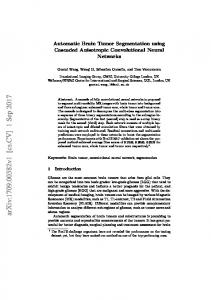
Fig. 3. Effect of the different proposed geometric constraints. Whereas the disjoint constraint (a)+(b) can be used to remove overlaps between initial segmentations, the template constraint (c) can bind the level set zero-crossing to the initial one in a locationspecific manner. With the proximity constraint (d), coincidence of shared boundaries can be imposed locally.

testing were used to train the learning-based pipeline, which were 313 boundary annotations for the liver and about 130 annotations for the other organs. After the the joint gradient descent had converged w.r.t. each energy of the level set segmentation, the final meshes were extracted from the level set maps via Marching Cubes. As error measure we first computed the shortest Euclidean distances between each result mesh and its corresponding annotated mesh at every vertex of the former as well as every vertex of the latter, and then averaged all such distances. The results in Table 1 show that the presented segmentation system yields state-of-the-art accuracies ranging from 1.17mm average surface error for left kidney to 2.89mm for the liver. Thereby the proposed level set segmentation contributes with an improvement of 20% for the liver, 30% for the left lung and left kidney, and 40% for the right lung and right kidney. Average run-times for the full detection pipeline is 2–3 min, which includes about 1 min for the only coarsely multi-threaded level set stage on a 2.0 GHz eight-core Xeon machine. Table 1. Symmetric surface errors using machine learning-based segmentation and after applying level set-based refinement Sym. surface error (mm)

Mean Std.dev. Median Worst 80% # cases

Liver, learning-based only Liver, level set-refined

3.5 2.9

1.7 1.7

3 2.6

4.0 3.6

100 100

Left lung, learning-based only Left lung, level set-refined

2.1 1.5

0.5 0.3

1.9 1.4

2.5 1.7

60 60

Right lung, learning-based only Right lung, level set-refined

2.7 1.6

0.9 0.6

2.4 1.5

3.0 1.8

60 60

Right kidney, learning-based only 1.9 Right kidney, level set-refined 1.1

0.9 0.9

1.8 0.8

2.0 3.9

10 10

Left kidney, learning-based only Left kidney, level set-refined

1.0 1.0

1.7 1.0

2.3 1.9

10 10

1.9 1.3

Automatic Multi-organ Segmentation

4

345

Conclusion

In our experiments we found the proposed algorithm to combine the robustness and speed of a machine learning approach with the high accuracy and advantageous distance map representation of a level set approach. Furthermore, the novel level set constraints allow to impose region-specific geometrical priors in the refinement stage. Yet the involved localized weights, as well as the global ones, need to be set manually in one or more parameter tuning sessions. One approach to automatize this step could be to minimize a sum energies in Equ. (8) over a set of fixed shapes gained from the learning-based stage with respect to these parameters. Finally, our experimental results show state-of-the-art accuracy and robustness of the proposed algorithm for five different organs on various unseen data sets.

References 1. Chan, T.F., Vese, L.A.: Active Contours without Edges. IEEE Trans. on Image Processing 10(2), 266–277 (2001) 2. Cremers, D., Rousson, M., Deriche, R.: A Review of Statistical Approaches to Level Set Segmentation: Integrating Color, Texture, Motion and Shape. IJCV 72(2), 195– 215 (2007) 3. Kohlberger, T., Uzunbas, G., Alvino, C., Kadir, T., Slosman, D., Funka-Lea, G.: Organ Segmentation with Level Sets Using Local Shape and Appearance Priors. In: Yang, G.-Z., Hawkes, D., Rueckert, D., Noble, A., Taylor, C. (eds.) MICCAI 2009. LNCS, vol. 5762, pp. 34–42. Springer, Heidelberg (2009) 4. Ling, H., Zhou, S.K., Zheng, Y., Georgescu, B., Suehling, M., Comaniciu, D.: Hierarchical, Learning-based Automatic Liver Segmentation. In: CVPR 2008, pp. 1–8. IEEE Press, New York (2008) 5. Liu, D., Zhou, S.K., Bernhardt, D., Comaniciu, D.: Search Strategies for Multiple Landmark Detection by Submodular Maximization. In: CVPR 2010, pp. 2831– 2838. IEEE Press, New York (2010) 6. Mansouri, A.-R., Mitiche, A., V´ azquez, C.: Multiregion Competition: A Level Set Extension of Region Competition to Multiple Region Image Partitioning. Computer Vision and Image Understanding 101(3), 137–150 (2005) 7. Paragios, N.: A Variational Approach for the Segmentation of the Left Ventricle in Cardiac Image Analysis. IJCV 50(3), 345–362 (2002) 8. Rousson, M., Paragios, N.: Shape Priors for Level Set Representations. In: Heyden, A., Sparr, G., Nielsen, M., Johansen, P. (eds.) ECCV 2002. LNCS, vol. 2351, pp. 78–92. Springer, Heidelberg (2002) 9. Tu, Z.: Probabilistic Boosting-Tree: Learning Discriminative Models for Classification, Recognition, and Clustering. In: ICCV 2005, vol. 2, pp. 1589–1596. IEEE Press, New York (2005) 10. Zheng, Y., Barbu, A., Georgescu, B., Scheuering, M., Comaniciu, D.: FourChamber Heart Modeling and Automatic Segmentation for 3-D Cardiac CT Volumes Using Marginal Space Learning and Steerable Features. IEEE Trans. on Medical Imaging 27(11), 1668–1681 (2008)