to automate this procedure and to generalize the derivation of ... Corresponding email: ..... are sent. Using the proposed notation, the derivation of the parame-.
Automatic Centralized Controller Design for Modular and Reconfigurable Robot Manipulators Andrea Giusti and Matthias Althoff Abstract— We address the problem of controlling modular robot manipulators. The challenge of modular-robot control is that the overall system dynamics are unknown due to its flexible composition from given modules. Most previous work has faced this problem by designing decentralized controllers. Simple decentralized controllers do not guarantee global asymptotic stability without knowledge of the overall system dynamics and alternative versions involving communication with neighboring modules result in complicated control concepts. Our approach is completely different: we store parameters regarding the dynamics and kinematics of each module and a unique identification number in itself. After finishing the assembly of the modules, the parameters are gathered in a central controller, which also detects the configuration using the identification numbers. Our centralized controller uses this information to synthesize modelbased control laws on-the-fly as if the full system dynamics are known beforehand. We introduce a novel and compact notation to automate this procedure and to generalize the derivation of the kinematic and dynamic model for heterogeneous modules. Finally, a possible application is shown using simulations.
I. INTRODUCTION Reconfigurable and modular robot manipulators are mechatronic systems composed of interchangeable modules. The modular nature of these systems allows them to be adapted for different applications, which is a clear advantage with respect to fixed-structure robots. This is especially useful in ultra-flexible environments, e.g. search and rescue operations, space explorations, service robots and robots for human-robot cooperation in manufacturing. In general, modular robots meet the different needs of the users through reconfigurations. Furthermore, modularity is also useful for robot manufacturers to reduce the number of parts as different robots can be assembled from a small set of modules. This makes it possible to provide a huge portfolio consisting of e.g. Selective Compliance Assembly Robotic Arm (SCARA) robots and anthropomorphic robots with a few standard modules. In the last three decades several modular robot manipulators have been developed, for instance the RMMS [1], TOMMS [2], IRIS [3], PolyBot [4] and a spring assisted reconfigurable modular robot [5]. The high versatility of the modular and reconfigurable robot manipulators leads to several challenges, especially for the design of the control system. Considering arbitrary configurations of a nonuniform set of modules, an enormous number of different dynamic systems can be obtained, challenging the control design. The authors are with the Department of Computer Science, Technische Universit¨at M¨unchen, 85748 Garching, Germany. Corresponding email:
{giusti, althoff}@in.tum.de
We present a new idea for controlling modular and reconfigurable robot manipulators based on distributed data stored in each module using a centralized control approach. After assembly of the modules, the modular information is collected by the central control unit, which automatically generates a centralized and model-based control law with guaranteed global asymptotic stability. The control design for modular robot manipulators has been a longstanding problem in research. Most work has mainly focused on decentralized control approaches. Adaptive decentralized control methods for modular robots are presented in e.g. [6], [7]. In the former the dynamic model of each subsystem is approximated to cancel the couplings and in the latter the parameters of distributed proportionalintegral-differential (PID) controllers are adjusted on-line. A decentralized control method for modular and reconfigurable manipulators is developed in [8] based on joint torque measurements for automatic compensation of the coupling effects. A decentralized and robust control method is presented in [9] that increases the performance with respect to a PID controller. A method for precision control of modular and reconfigurable manipulators with guaranteed stability is presented in [10] using the virtual decomposition approach. A hybrid architecture for centralized and decentralized operations is proposed in [11], where the authors consider the decentralized approach for controlling the manipulator dynamics. Even though satisfying results have been achieved with advanced decentralized schemes, every decentralized control method can be considered as a special case of a centralized one. In principle, it is always possible to design a centralized controller with performance equal to or better than a decentralized control scheme. Especially when fast trajectory tracking is required or direct drive actuation is employed, centralized control schemes are superior compared to decentralized controllers since subsystem couplings can be compensated instead of treating them as disturbance [12]. Moreover, centralized architectures are also beneficial for optimal control, compliance and impedance control [12], dynamic scaling of trajectories [13], and failure detection [14]. Automatic generation of complete models from modules has previously been investigated in [15]. In [16] a centralized control design is considered. In contrast to our work, these approaches assume similar modules with symmetric geometry and a central database storing the information of all modules, which is impractical as discussed later. A previous approach that considered the storage of information in the
modules is described in [17], where the automatic derivation of kinematics is considered for joint modules with similar geometry. Our proposed approach is different because we consider modules with arbitrary kinematic and dynamic parameters stored in each module. Our kinematic modeling procedure is based on the Denavit-Hartenberg convention, which is related to the works in [18]–[20]. In these works, it is required to store homogeneous transformation matrices in a central database, which is not a requirement of our approach. We introduce a novel notation and an extension of the standard Denavit-Hartenberg convention that simplifies the automatic procedure for obtaining the relative parameters, especially when considering prismatic joints. Moreover, our approach also considers dynamics with the final goal of automatically designing model-based control laws. The main novelties that this work introduces are summarized as follows: i) none of the cited approaches have considered distributing information to the modules to enable and/or automate the centralized and model-based controller design after information collection; ii) our automatic controller design approach is generalized and can thus be applied when modules are heterogeneous (e.g. with different shapes and dynamic parameters); iii) we provide a systematic method to characterize modules using a novel notation and an extension of the standard DenavitHartenberg convention; iv) our approach does not require symbolic computation for the automatic centralized controller design of reconfigurable modular robot manipulators. The paper is organized as follows. In Sec. II we describe the control problem for modular robot manipulators in detail. The proposed method is presented in Sec. III followed by simulation results in Sec. IV.
are respectively the vectors of friction and gravity terms, finally u ∈ RN is the vector of the actuation forces/torques. We consider only viscous friction without loss of generality of our presented approach. The matrices and vectors of the dynamic model in (1) are different for various compositions of the manipulator and type of modules. We face the problem of automatically generating a centralized controller in the joint space that guarantees global asymptotic stability after a reconfiguration: lim ke (t)k = 0,
t→∞
where ke (t)k = kqr (t) − q (t)k is the Euclidean norm of the error vector in the joint space and qr (t) is the differentiable (of class C2 ) desired trajectory. We consider the development in time of this error as a performance indicator. III. PROPOSED METHOD Our proposed approach is illustrated in Fig. 1: each module is first characterized according to our proposed notation, which is stored within the module. After the selection of the modules and the manual assembly of the robot, the automatic controller design process starts. First, information related to the kinematics, dynamics and a unique identification number (e.g. the Media Access Control (MAC) address) are collected from all modules by the central control unit. Next, the centralized controller is automatically generated to let the robot operate with guaranteed motion control performance. Characterization of each module and storage of the information in itself Manual Assembly
II. PROBLEM DESCRIPTION We consider a modular and reconfigurable robot manipulator composed of serially connected rigid links. Throughout this paper we also assume that: a) each module includes a rigid proximal part, a rigid joint, and a rigid distal part (see Fig. 3); b) the connectors are standardized and allow the assembly of two subsequent modules at only one relative orientation; c) the motor inertia effects are not considered for a succinct presentation of the material since this does not affect the basic idea of our approach. For a concise presentation of our method, we further exclude modules that do not introduce a new degree of freedom (e.g. link modules). The consideration of such modules is trivial, as it becomes evident later. A reconfigurable modular robot manipulator with N serially connected modules constitutes an open kinematic chain and has the following dynamic model (see [12]): ˙ q˙ + f (q) ˙ + g (q) = u, M (q) q¨ + C (q, q)
(1)
where q ∈ RN is the vector of the generalized coordinates, M (q) ∈ RNxN is the symmetric and positive definite mass ˙ q˙ (with C (q, q) ˙ ∈ RNxN ) is the vector of the matrix, C (q, q) ˙ ∈ RN and g (q) ∈ RN Coriolis and centrifugal terms, f (q)
select modules
Automatic Controller Design system in operation information collection model-based controller generation (automatic)
Fig. 1.
Illustration of the proposed approach.
The information of the modules can be stored in two ways: i) using a centralized database with stored information of all the modules that can be used; ii) using distributed memory to store information of a module in the module itself. Obviously, the latter option is preferred since the first one requires database updates when new modules are created and additionally requires storage of all possible modules (leading to storage and legacy issues).
We propose a tree structure as a suitable topology of the communication network for modular robotic manipulators with an open kinematic chain. The tree-structured network supports serial and branch-structured manipulators and is composed of a coordinator associated with the central control unit, routers associated with the intermediate modules and end-devices associated with the end effectors. In this structure, each module allows the coordinator to get measurements (e.g. joint position and velocity), set input commands to the actuators and set/get data in/from its local memory database (e.g. dynamic and kinematic parameters and type of joints). Moreover, collecting additional information (e.g. the routing tables) makes it possible for the central control unit to detect the robot configuration. Appropriate information from the modules enables the central control unit to automatically compute the forward kinematics based on an extended Denavit and Hartenberg convention as is described in III-A and the dynamic model with the recursive Newton-Euler method as presented in III-B. Finally, model-based control laws are automatically synthesized as discussed in III-C. A. Forward Kinematics using Modular Information The forward kinematics allows obtaining the pose of the end effector (position and orientation) given the joint positions. For an open kinematic chain the forward kinematics is commonly derived in a recursive way, by multiplying the homogeneous transformation matrices that relate the frame of reference of each link to the previous one. A systematic method for the assignment of the frame of reference of each link is the Denavit-Hartenberg (D-H) convention [21], which we briefly recall. Consider that the ith link of the robot has a body-fixed frame of reference with axes xi , yi and zi . According to the standard D-H convention (see Fig. 2), zi is aligned with the axis of the joint at the connection with link i + 1. The xi axis is chosen along the common normal between the axis zi−1 and zi pointing toward the link i + 1. The origin of the frame i is set at the intersection of the common normal with zi . Finally, the yi axis completes the righthanded coordinate system. Once the frames of reference are assigned, four parameters are introduced to define the relative transformation of coordinates: ai , di , αi , θi . As shown in Fig. 2, ai is the distance along xi between the origin of the frame i′ and i, di is the distance along zi−1 between the origin of the frame i − 1 and i′ , αi is the angle between the axis zi−1 and zi around xi and θi the angle between xi−1 and xi around zi−1 (the angles are positive counterclockwise). The only variable parameter is di when the joint is prismatic and θi when it is revolute [12]. Considering that our proposed approach is automatic and that the standard D-H convention is not unique, we extend it to handle some particular cases that need special consideration (see Fig. 2): •
when the z axes intersect, the xi unit vector is obtained from the cross product between them;
PJi linki
PJi−1
αi
pi ni−1
zi′
yi′ di yi−1
xi′
oi ′
ai
θi
ni zi
yi oi
xi
zi−1 oi−1 xi−1
Fig. 2.
Representation of a link showing the parameters for kinematics.
when the z axes are parallel the xi unit vector is set along the common normal between them and the origin oi is set at the joint connection PJi ; • when the z axes are superimposed the xi unit vector is aligned with xi−1 and the origin oi is set at the joint connection PJi . In order to automate the derivation of the four D-H parameters for each link (D-H table), we introduce two additional parameters associated to each link. These are obtained on the basis of the link geometry: pi and ni , and are the z coordinates of the point PJi−1 from oi′ and of the point PJi from oi , respectively (see Fig. 2). Using these two parameters, di can be recursively computed as: •
di = ni−1 − pi (revolute joint), di = ni−1 − pi + qi (prismatic joint), where qi is the joint displacement. Additionally, in order to capture the constant angular offset that can be present between xi−1 and xi when the joint is in its zero position and when it is prismatic, an additional parameter γi is introduced. With this addition, the D-H parameter θi is:
θi = γi + qi (revolute joint), θi = γi (prismatic joint). In the following, we introduce a notation to characterize arbitrary modules and the automatic procedure to obtain the parameters of the extended D-H convention (ai , αi , pi , ni , γi ) for each link of an assembled manipulator. Let us consider the exemplary module shown in Fig. 3(a). This module is composed of an input connector, a joint and an output connector. To define the new notation, we first have to decompose the module into a proximal (pl) and a distal part (dl). These parts are shown in Fig. 3(c) and Fig. 3(b), respectively. In this description, we consider modules with only one degree of freedom without loss of generality because more complex modules can be modeled as a series of those considered, by setting the relevant parameters to zero. The first step to characterize the module is to fix a frame of reference for the proximal part and the distal part. These two frames are located in the center of the interfaces of the respective connectors. The axes xin and xout are positioned
Output connector
Joint Input connector
(a) zout
oout δ dl
yout (b)
PJ
xout pdl
α dl ndl z′dl ′ xdl
y′dl
zin
oin
z′′dl
y′′dl
o′′dl
δj
o′dl
α pl
adl
′′ xdl
PJ
yin
(c)
xin z′pl
p pl o′pl
y′pl
x′pl
δ pl
z′′pl a pl
o′′pl
y′′pl
n pl
x′′pl
Fig. 3. Kinematic notation for module characterization. The connectors are indicated in light-grey color, (a) is the entire module, (b) the distal part and (c) the proximal part.
along a unique and standardized direction on the connection plane. The z axes are normal to the respective connector planes, zin points in towards the input connector and zout points outwards from the output one (see Fig. 3). The axes yin and yout are selected to complete the respective righthanded frames of reference. According to our notation we characterize both the proximal and the distal part with a set of parameters. To obtain these parameters, the same approach of the extended D-H convention described previously is applied. Accordingly, we obtain four parameters for the proximal part: a pl , α pl , p pl , n pl , and for the distal part: adl , α dl , pdl and ndl . Regarding the proximal part illustrated in Fig. 3(c), two auxiliary frames are considered. The first one has its origin at o′pl , the intersection of the common normal between zin and the joint axis with zin . The axis x′pl is set along the common normal pointing toward the distal part, z′pl is set along zin and y′pl completes the right-handed frame of reference. The second auxiliary frame has its origin in o′′pl at the intersection of the common normal with the joint axis, its axis x′′pl is set along the common normal and points toward the distal part, z′′pl is set along the joint axis and finally y′′pl completes the right-handed frame of reference. The four parameters for the proximal part have the following meanings: •
a pl is the distance between o′pl and o′′pl along the common normal;
α pl is the angle between the axis zin and the joint axis around x′′pl ; • p pl is the z coordinate of the input connection point oin from o′pl ; • n pl is the z coordinate of the joint connection point PJ from o′′pl . For the distal part illustrated in Fig. 3(b), two auxiliary frames are analogously introduced. The four parameters for the distal part have similar meanings: • adl is the distance between o′dl and o′′ dl , along the common normal; • α dl is the angle between the joint axis and zout around ′′ ; xdl • pdl is the z coordinate of the joint connection point PJ from o′dl ; • ndl is the z coordinate of the output connection point oout from o′′dl . Finally, three additional parameters are required: δ pl , δ dl , j δ . As shown in Fig. 3(c) and (b): δ pl is the angle between ′′ and x , and finally x′pl and xin , δ dl is the angle between xdl out ′ j ′′ δ is the angle between x pl and xdl when the joint is in its zero position (all the angles of this notation are positive counterclockwise). Particular cases of the relative orientation between the z axes (e.g. parallel, intersect or overlap) are handled similarly to the previously described extension of the standard D-H convention. The connection points to consider are: oin and PJ (proximal part); PJ and oout (distal part). We collect the parameters required to characterize a module for kinematics in Tab.I. •
TABLE I I NFORMATION STORED IN EACH MODULE FOR KINEMATICS . Proximal Distal Joint
a pl adl
δj
α pl α dl
p pl pdl
δ pl n pl δ dl ndl Joint type
It is worth noting that the same approach can be applied to modules with multiple input and output connectors. In those cases, a set of parameters for each realizable combination of the connectors is required and has to be stored in the module. When the information is forwarded to the central control unit, the set of parameters corresponding to the connectors in use are sent. Using the proposed notation, the derivation of the parameters of the extended D-H convention for each link (ai , αi , pi , ni , γi ) can be automated. Let us assume that the ith connection between a module i − 1 and a module i is established. In order to obtain the parameters for the link, we require the homogeneous transformation matrix Fi of a frame oriented as the D-H one located at PJi (see Fig. 2) with respect to a frame parallel to the first auxiliary frame of the distal part of the module i − 1 with origin PJi−1 (see Fig. 3(b)). From now on, we use a compact notation to indicate operations with homogenous transformation matrices. For instance: Tk (·)/Rk (·) are homogeneous transformations that represent
the translation/rotation along/around the k axis. Using the parameters that characterize subsequent modules, we first calculate an auxiliary matrix F′i . This matrix describes the transformation of a frame with origin at PJi , parallel to the second auxiliary frame of the proximal part of module i, with respect to a frame parallel to the first auxiliary frame of the distal part of module i − 1 and with origin at PJi−1 . It is calculated as: dl dl dl F′i =Tz (−pdl i−1 )Tx (ai−1 )Rx (αi−1 )Tz (ni−1 )
(2)
i. When the axes overlap: φi = 0. ii. When the axes are parallel: φi = arctan(vy /vx ), from � �T ′ V = vx vy vz = R′T i Ui . iii. When the axes are skew or intersect: φi = arctan(vy /vx ), from � �T ′ ′ = R′T V = vx vy vz i V and V = zi × zi−1 . as:
uxi uyi . uzi 1
(3)
The same transformation of Fi can be expressed in terms of the parameters of a link and an auxiliary rotation (φ ′ ) as: Li =Tz (−pi )Rz (φi′ )Tx (ai )Rx (αi )Tz (ni ) Cφi′ −Cαi Sφi′ Sαi Sφi′ aiCφi′ + ni Sαi Sφi′ Sφ ′ Cα Cφ ′ −Sα Cφ ′ ai Sφ ′ − ni Sα Cφ ′ i i i i i i i i = 0 Cαi niCαi − pi Sαi 0 0 0 1
, (4)
where Sε /Cε are the abbreviations of sine/cosine of an angle ε . Equating (4) and (3), the parameters of our extended D-H convention for the ith connection (or link) can be inferred: ai = uxi rxi + uyi ryi ,
αi = arctan(szi /tzi ), φi′
z }| { j − φi−1 . γi = arctan(ryi /rxi ) + δi−1
If szi = 0: ni = 0, B. Dynamic Model from Modular Information
In order to complete the synthesis matrix Fi , an additional possible rotation φi around zi is considered. In fact, we need to align the x axis according to our extended D-H convention. With the transformation of (2) we only reached a frame located at PJi with the orientation of the second auxiliary frame of the proximal part of module i. An additional rotation around z may be required to bring this frame parallel to the D-H one. In order to find this angle, we have to consider three possible cases for the joint axes. The detection of the case that occurs is performed using U′i , and the unit vector of the z axis in R′i , which contains the information of the relative orientation of two subsequent joint axes.
txi tyi tz i 0
(uxi ryi − uyi rxi ) , szi (uxi tzi ryi − uzi szi − uyi tzi rxi ) . pi = s zi ni =
pi = −uzi .
dl − δipl )Tz (−pipl )Tx (aipl )Rx (αipl )Tz (nipl ) Rz (δi−1 � � ′ Ri U′i . = 0T 1
The synthesis matrix is completed rxi sxi ryi syi Fi = F′i Rz (φi ) = rzi szi 0 0
If szi 6= 0:
The problem of deriving the dynamic model of a rigid link manipulator is usually solved either with Lagrangian formulation [22] or recursive Newton-Euler (N-E) methods [23]. A comparison of the methods for the derivation of the equations of motion of a rigid link manipulator is in [22]. A computationally efficient variant of the Newton-Euler method has first been proposed in [23] with a complexity � that grows linearly with the number of the joints O(N) . Subsequently, enhanced versions of this algorithm have been presented in e.g. [24], [25]. A review on methods for robot dynamics can be found in [26]. The recursive N-E algorithm studies the manipulator link by link and is composed of two recursions, one for kinematics (forward recursion) and one for forces and torques (backward recursion). It can be used either with symbolic computations to obtain the closed form dynamic model or with numerical ones for control as described later. We consider the recursive N-E algorithm of [12] without motor inertia effects. Similar to the kinematics, we provide a systematic approach to characterize the modules for dynamics. The set of required parameters for each module is presented as well as the procedure to synthesize them for each established connection. For each link of the manipulator (see Fig. 4), a body-fixed frame of reference with origin in Di is considered. We consider this frame to have the same orientation as the D-H one so that the results of the forward kinematics are exploited to infer relative orientation of subsequent links. With reference to the generic link of Fig. 4, the vector from Di−1 to Di is riDi−1 ,Di and the vector from Di to Ci (the center of mass) is riDi ,Ci . In addition to these vectors, the mass mi , the inertia tensor Iii and the viscous damping coefficient of the joint FJi−1 are also required for the algorithm. The superscript of all the vectors indicates in which frame of reference they are expressed. Similarly to the kinematics, a synthesis procedure is required for the dynamics based on modular information. A graphical representation of the ith connection involving dynamic parameters is shown in Fig. 5. In our approach, the required parameters for dynamics are expressed in the output frame for the distal part and in the input frame for the proximal part. For each module, beyond the mass for both the distal (mdl ) and the proximal part (m pl ), we require their in inertia tensors: Iout dl , I pl , and the coordinates of the centers of out in mass: rCdl , rCpl , expressed in the output and the input frame, respectively.
riDi−1 ,Di
zi−1
Di−1 Fig. 4.
yi zi
0 S(U) = uz −uy
xi Di riDi ,Ci
Ci
Representation of a link for dynamic related parameters.
ith connection z oini ini xini out
ini rCpl i
PJi
Cpli
youti−1
PJi−1
Using this notation, when the ith connection is realized, the output frame of module i − 1 and the input frame of module i match. We denote the matched frame as “io”. The synthesis of the total mass of the link mi , the coordinates of its center of mass rCioi and the inertia tensor Iio i can thus be automated: pl io out in mi = mdl i−1 + mi , Ii = Idli−1 + I pli ,
=
pl in out mdl i−1 rCdli−1 + mi rCpli
mi
.
Our proposed automatic procedure transforms these quantities to be expressed in a frame parallel to the D-H one and located at Di for each realized link i (see Fig. 4). Since the kinematic parameters are known, these transformations of coordinates are performed using homogeneous transformations and Steiner’s theorem [12] for the inertia tensor. The coordinates of the center of mass are computed as: � � � � i � �−1 rCio rDi ,Ci i , = Aio i 1 1 where pl pl pl pl pl Aio i = Rz (−δi )Tz (−pi )Tx (ai )Rx (αi )Tz (ni )Rz (φi ) � � io Ri Uio i . = 0T 1
The inertia tensor in computed as: � � T T i T io i io io Iio Iii = Rio i −mi S (rCi )S(rCi ) Ri +mi S (rDi ,Ci )S(rDi ,Ci ), i where S(·) is an anti-symmetric matrix:
uz
�T
.
The last parameter that needs to be synthesized for each constituted link is riDi−1 ,Di . Also for this vector we can use homogeneous transformations with the synthesized kinematic parameters: Aii−1 = Tz (−pi + qi )Rz (γi )Tx (ai )Rx (αi )Tz (ni ) (prism. joint), and finally � i � i−1 �−1 Ri−1 i Ai−1 = Ai = 0T
Uii−1 1
�
, riDi−1 ,Di = −Uii−1 .
TABLE II I NFORMATION TO STORE IN THE MODULES FOR DYNAMICS .
oouti−1
Fig. 5. Representation of a connection involving parameters for dynamics. Connectors are indicated in light-grey color.
rCioi
uy
We store the additional parameters in each module for the dynamics as collected in Tab. II.
xouti−1 Cdli−1
uy � −ux , with U = ux 0
Aii−1 = Tz (−pi )Rz (γi + qi )Tx (ai )Rx (αi )Tz (ni ) (rev. joint),
yini
zouti−1
rCdli−1 i−1
−uz 0 ux
Proximal Distal Joint
m pl mdl FJ
Iin pl Iout dl
in rCpl out rCdl
C. Centralized Controller Design The procedures described for automatic derivation of kinematics and dynamics enable the automatic generation of model-based control laws using the modular information in Tab. I and II. Our proposed centralized controller for modular and reconfigurable robot manipulators takes as input ˙ the reference the position vector (q), the velocity vector (q), trajectory (qr , q˙ r , q¨ r ) and finally the array of structures containing the information of the modules: ModRob. The array of structures ModRob contains the information of Tab. I and II for each module. The output is the closed loop force/torque command, which guarantees global asymptotic stability. In order to realize the model-based control laws, we ˙ q, ¨ ModRob), have implemented a function u = NEmod (q, q, that performs the recursive N-E algorithm using ModRob as described in Sec. III-A and III-B and returns the force/torque commands. We have implemented the automatic generation of two model-based control laws: proportional and derivative (PD) control with gravity compensation and computed torque control. Computed torque control is one of the most effective centralized and model-based control methods for robotic manipulators with rigid links. Assuming perfect knowledge of the system dynamics, computed torque linearizes the model of (1) by compensating the nonlinear and coupling terms through feedback. The control law is completed by assigning an input (υ ) to the linearized system that guarantees asymptotically stable dynamics of the error in joint space [27]. The PD control with gravity compensation [12] is suitable for point to point motion and is designed to compensate the gravitational terms of the dynamic model and to include
xout
zout xout
zin
zin
zin
xin
xin
1 0.8 0.6 0.4 0.2 0 -0.2 0
TABLE III I NFORMATION OF THE MODULES USED FOR SIMULATION . Parameter a pl (m) α pl (rad) p pl (m) n pl (m) δ pl (rad) adl (m) α dl (rad) pdl (m) ndl (m) δ dl (rad) δ j (rad) Joint Type in (m) rCpl m pl (kg)� 2 Iin pl kgm (diagonal) out (m) rCdl mdl (kg) � Iout kgm2 dl (diagonal) FJ (Nms)
a 0 −π /2 −0.1 0 0 0 −π /2 0 0.1 0 π Rev. [0 0 0.05]T 0.5 10−3 · [2 2 0.65] [0 0 − 0.05]T 0.5 10−3 · [2 2 0.65] 3
b 0 0 −0.1 0 0 0 0 −0.1 0 0 0 Rev. [0 0 0.05]T 0.5 10−3 · [2 2 0.65] [0 0 − 0.05]T 0.5 10−3 · [2 2 0.65] 3
c 0 0 −0.1 0 0 0 0 −0.05 0 0 0 Prism. [0 0 0.05]T 0.5 10−3 · [2 2 0.65] [0 0 − 0.025]T 0.25 10−3 · [0.36 0.36 0.31] 3
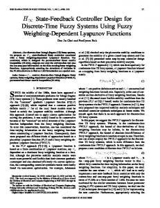
a linear feedback control law for positions and velocities. Assuming perfect knowledge of the gravitational term, PD control with gravity compensation guarantees global and asymptotic stability for any desired constant equilibrium posture [12]. We obtain the compensating commands for the control laws numerically by varying appropriate numerical arguments to the function NEmod . For example, the numerical vector of the gravitational terms used for PD control with gravity compensation is computed as g (q) = NEmod (q, 0, 0, ModRob) and the closed loop command of the computed torque control is computed numerically as ˙ υ , ModRob) where q, q˙ are the current ucl = NEmod (q, q, numerical vectors of positions and velocities. IV. SIMULATION RESULTS A point to point motion in the joint space is simulated for a configuration using a given set of modules. We show and compare results of the automatically generated control laws: PD control with gravity compensation and computed torque control. Gaussian measurement noise and input disturbance are included. We consider these distributions with zero mean and standard deviation of σn = 0.03 for measurements of joint positions (rad and m) and velocities (rad/s and m/s)
1
2
0.5
1
1.5
2
2.5
time (s)
�
e (t) /qr t f in
Fig. 6. Representation of the modules for illustrative purpose used for simulations. Connectors are indicated in light-grey color.
0.4 0.2 0
0
time (s)
Fig. 7. Simulation using PD with gravity compensation controller. The dashed lines represent the desired trajectories.
q1:4 (t) (rad)
c
0.5
0.6
1 0.8 0.6 0.4 0.2 0 -0.2 1.5
2
1 0.8 0.6 0.4 0.2 0 -0.2 2.5
1.5
2
2.5
Module 01 Module 02 Module 03 Module 04 Module 05
0
0.5
1
0.5
1
time (s)
0.6
�
e (t) /qr t f in
b
a
1.5
1 0.8 0.6 0.4 0.2 0 -0.2 2.5
Module 01 Module 02 Module 03 Module 04 Module 05
q5 (t) (m)
zout
q5 (t) (m)
xin
xout
q1:4 (t) (rad)
zout
0.4 0.2 0
0
time (s)
Fig. 8. Simulation using computed torque controller. The dashed lines represent the desired trajectories.
and σu = 0.3 for the input forces/torques (N and Nm). We perform the simulations using three kind of modules shown in Fig. 6: a, b (revolute joints) and c (prismatic joint). The parameters of the modules used for these examples are collected in Tab. III. Using these modules we build a configuration composed of five modules: [b-a-b-a-c]. The trajectory of each joint is designed with a quintic polynomial. The coefficients have been selected to guarantee zero initial/final velocity and zero initial/final acceleration. The final time of the planned motion is t f in = 1s with a starting time tin = 0s. The joints start from zero to reach the final positions: q(t f in ) = [0.2, 0.4, 0.6, 0.8, 0.1]T . The simulations are performed using the following gain matrices [12] of the controllers: K p = 250 I and Kd = 30 I, where I is the identity matrix of proper dimensions. As shown in Fig. 7 and Fig. 8, computed torque control has better performance observing the development in time of the Euclidean norm of the error. In these figures, we show the error vector as a fraction of the respective final positions of the trajectories for normalized presentation in one plot. V. CONCLUSIONS We present a systematic and effective approach for centralized control of modular and reconfigurable robot manip-
ulators. To the best knowledge of the authors, none of the approaches presented in the literature so far have considered distributing information to the modules to automatically generate a pure model-based centralized controller, especially when considering heterogeneous modules. This idea paves the way for future modular and reconfigurable robotic systems with performance and capabilities that approach those of fixed structure ones from a control perspective. Having the possibility to auto-generate a model-based centralized controller with guaranteed asymptotic stability for a non-uniform set of modules, the central control unit does not require a large database and successive updates. Fast reconfiguration with guaranteed stable operations and motion control performance ensures hyper-flexibility of the robotic system. A drawback of this approach compared to conventional methods for controlling modular robot manipulators is the necessary storage of information in the modules that may increase manufacturing costs. Additionally, if self-detection of the configuration were required, network solutions that support a tree-structured topology would be needed. A communication bus (e.g. CAN bus) could also be suitable but additional communication lines have to be employed as described in [17]. However, we believe that the cost savings from standardization of modular robots would outweigh such cost increases. Furthermore, the automated generation of the controller with guaranteed motion control performance would reduce the time and costs required for commissioning the robot after assembling or reconfiguration. An important continuation of this work is the introduction of robustness for uncertain modular information, elasticity in the joints and measurement noise, especially because in future works this control approach will be implemented on a real robot. ACKNOWLEDGMENT The research leading to these results has received funding from the People Programme (Marie Curie Actions) of the European Union’s Seventh Framework Programme FP7/20072013/ under REA grant agreement number 608022. R EFERENCES [1] D. Schmitz, P. Khosla, and T. Kanade, “The CMU reconfigurable modular manipulator system,” Inst. Software Res., Carnegie Mellon Univ., Pittsburgh, PA, USA, CMU-RI-TR-88-7, Tech. Rep., 1988. [2] T. Matsumaru, “Design and control of the modular robot system: TOMMS,” in Proc. 1995 IEEE Int. Conf. Robotics and Automation, vol. 2, May 1995, pp. 2125–2131. [3] R. Hui, N. Kircanski, A. Goldenberg, C. Zhou, P. Kuzan, J. Wiercienski, D. Gershon, and P. Sinha, “Design of the IRIS facility-a modular, reconfigurable and expandable robot test bed,” in Proc. 1993 IEEE Int. Conf. Robotics and Automation, vol. 3, May 1993, pp. 155–160. [4] M. Yim, D. Duff, and K. Roufas, “PolyBot: a modular reconfigurable robot,” in Proc. 2000 IEEE Int. Conf. Robotics and Automation, vol. 1, 2000, pp. 514–520. [5] G. Liu, Y. Liu, and A. Goldenberg, “Design, analysis, and control of a spring-assisted modular and reconfigurable robot,” IEEE/ASME Transactions on Mechatronics, vol. 16, no. 4, pp. 695–706, Aug 2011. [6] M. Zhu and Y. Li, “Decentralized adaptive fuzzy control for reconfigurable manipulators,” in 2008 IEEE Conference Robotics, Automation and Mechatronics, Sept 2008, pp. 404–409.
[7] W. Melek and A. Goldenberg, “Neurofuzzy control of modular and reconfigurable robots,” IEEE/ASME Transactions on Mechatronics, vol. 8, no. 3, pp. 381–389, Sept 2003. [8] G. Liu, S. Abdul, and A. Goldenberg, “Distributed modular and reconfigurable robot control with torque sensing,” in Proc. 2006 IEEE Int. Conf. Mechatronics and Automation, June 2006, pp. 384–389. [9] W. Li, Z. Melek and C. Clark, “Decentralized robust control of robot manipulators with harmonic drive transmission and application to modular and reconfigurable serial arms,” Robotics, vol. 27, pp. 291– 302, 2009. [10] W.-H. Zhu, T. Lamarche, E. Dupuis, D. Jameux, P. Barnard, and G. Liu, “Precision control of modular robot manipulators: The VDC approach with embedded FPGA,” IEEE Transactions on Robotics, vol. 29, no. 5, pp. 1162–1179, Oct 2013. [11] D. Wang, A. Goldenberg, and G. Liu, “Development of control system architecture for modular and re-configurable robot manipulators,” in ICMA 2007. Int. Conf. Mechatronics and Automation, Aug 2007, pp. 20–25. [12] B. Siciliano, L. Sciavicco, L. Villani, and G. Oriolo, Robotics: Modelling, Planning and Control. Springer, 2009. [13] J. Hollerbach, “Dynamic scaling of manipulator trajectories,” ASME Journal of Dynamic Systems, Measurement and Control, vol. 106, pp. 102–106, 1984. [14] A. De Luca and R. Mattone, “Actuator failure detection and isolation using generalized momenta,” in Proc. 2003 IEEE Int. Conf. Robotics and Automation, vol. 1, Sept 2003, pp. 634–639. [15] I. Chen, S. Yeo, G. Chen, and G. Yang, “Kernel for modular robot applications: Automatic modeling techniques,” The International Journal of Robotic Research, vol. 18, no. 2, pp. 225–242, 1999. [16] E. Meister, A. Gutenkunst, and P. Levi, “Dynamics and control of modular and self-reconfigurable robotic systems,” International Journal on Advances in Intelligent Systems, vol. 6, no. 1&2, pp. 66–78, 2013. [17] P. Xinan, W. Hongguang, J. Yong, and X. Jizhong, “Automatic kinematic modelling of a modular reconfigurable robot,” Transactions of the Institute of Measurement and Control, vol. 35, no. 7, pp. 922– 932, 2013. [18] L. Kelmar and P. Khosla, “Automatic generation of kinematics for a reconfigurable modular manipulator system,” in Proc. 1988 IEEE Int. Conf. Robotics and Automation, vol. 2, Apr 1988, pp. 663–668. [19] B. Benhabib, G. Zak, and M. Lipton, “A generalized kinematic modeling method for modular robots,” Journal of Robotic Systems, vol. 6, no. 5, pp. 545–571, 1989. [20] Z. Bi, W. Zhang, I. Chen, and S. Lang, “Automated generation of the D-H parameters for configuration design of modular manipulators,” Robotics and Computer-Integrated Manufacturing, vol. 23, pp. 553– 562, 2007. [21] J. Denavit and R. Hartenberg, “A kinematic notation of lower-pair mechanisms based on matrices,” ASME Journal of Applied Mechanics, vol. 22, pp. 215–221, 1955. [22] J. Hollerbach, “A recursive lagrangian formulation of maniputator dynamics and a comparative study of dynamics formulation complexity,” IEEE Transactions on Systems, Man and Cybernetics, vol. 10, no. 11, pp. 730–736, Nov 1980. [23] J. Luh, M. Walker, and R. Paul, “On-line computational scheme for mechanical manipulators,” ASME Journal of Dynamic Systems, Measurement and Control, vol. 102, pp. 468–474, 1980. [24] A. De Luca and L. Ferrajoli, “A modified Newton-Euler method for dynamic computations in robot fault detection and control,” in Proc. 2009 IEEE Int. Conf. Robotics and Automation, May 2009, pp. 3359– 3364. [25] L. Sciavicco, B. Siciliano, and L. Villani, “Lagrange and NewtonEuler dynamic modelling of a gear-driven rigid robot manipulator with inclusion of motor inertia effects,” Advanced Robotics, vol. 10, no. 3, pp. 317–334, 1996. [26] R. Featherstone and D. Orin, “Robot dynamics: equations and algorithms,” in Proc. 2000 IEEE Int. Conf. Robotics and Automation, vol. 1, 2000, pp. 826–834. [27] W. Chung, L.-C. Fu, and S.-H. Hsu, “Motion control,” in Handbook of Robotics, B. Siciliano and O. Khatib, Eds. Springer, 2008, pp. 133–159.