Automatic Feature Selection in Large-Scale System-Software Product Lines Andreas Ruprecht
Bernhard Heinloth
Daniel Lohmann
Friedrich-Alexander University Erlangen-Nuremberg, Germany {ruprecht, heinloth, lohmann}@cs.fau.de
Abstract
16000
System software can typically be configured at compile time via a comfortable feature-based interface to tailor its functionality towards a specific use case. However, with the growing number of features, this tailoring process becomes increasingly difficult: As a prominent example, the Linux kernel in v3.14 provides nearly 14 000 configuration options to choose from. Even developers of embedded systems refrain from trying to build a minimized distinctive kernel configuration for their device – and thereby waste memory and money for unneeded functionality. In this paper, we present an approach for the automatic use-case specific tailoring of system software for special-purpose embedded systems. We evaluate the effectiveness of our approach on the example of Linux by generating tailored kernels for well-known applications of the Rasperry Pi and a Google Nexus 4 smartphone. Compared to the original configurations, our approach leads to memory savings of 15–70 percent and requires only very little manual intervention.
14000
Features
12000 10000 8000 6000 4000
hardware features (in arch, drivers and sound)
2000 0
software features (everything else)
Linux kernel version
Figure 1. Linux feature growth 2005––2014
Categories and Subject Descriptors D.2.9 [Software Engineering]: Management – Software configuration management; D.4.7 [Operating Systems]: Organization and Design
appears to be inevitable, as it is mostly caused by advances in hardware: About 88 percent of all features directly deal with low-level hardware support (Figure 1). Especially embedded platforms, such as ARM, with many derivatives and short innovation cycles have become a driving force in this process. The consequence: When configuring a Linux kernel, developers are faced with an overwhelmingly large number of options. With thousands of features representing potential choices, finding the right set of optional features specifically needed for your system is a hard and time-consuming task that, furthermore, requires detailed knowledge about both, Linux and the platform in use. To suit as many customers and their hardware as possible, distributors ship a Linux kernel configuration with most optional features enabled. Instead of per-use-case tailoring, we are practically back to onesize-fits-all solutions. One may consider this as a pragmatic approach for workstations with disk sizes of 1 TB or more and several GB of RAM. However, if you need system-software for a special-purpose embedded system, you want it to be as small as possible. Currently, Linux is already used in smartphones and is the prevailing operating system installed on mini computers like the Raspberry Pi. There are however much more specific use cases for small-scale systems which could be driven by Linux, such as home automation systems or electronic control units used in the automotive industry, where low per-unit costs are a crucial requirement [4]. In the case of Linux, this has led to the development of special minimized versions like uLinux [8] and tinyLinux [14], but these make many assumptions about your system and its usage, trading flexibility for size. Moreover, even on those systems a lot of effort is required by the providing developer to find a valid minimal con-
General Terms Experimentation, Management, Measurement Keywords Software Tailoring, Feature Selection, Software Product Lines, Linux
1.
software hardware all
Introduction
Most system software can be configured at compile time to tailor it with respect to a broad range of supported hardware architectures and application domains. The most prominent example is the Linux operating-system family, which in v3.14 offers close to 14 000 configurable features across 26 architectures. But also many other pieces of system software, such as BusyBox [5] (UNIX core utilities), CoreBoot [3] (BIOS/UEFI firmware), or eCos [15] (operating system), already provide hundreds to thousands of – mostly optional – features [1]. These numbers are subject to an ongoing growth: Between 2005 and 2014, the number of configurable features in Linux has grown by 10-–20 percent every year! This growth
Permission to make digital or hard copies of all or part of this work for personal or classroom use is granted without feecopies provided thatorcopies notwork madefor or personal distributed Permission to make digital or hard of all part ofarethis or for profit oruse commercial andprovided that copies thisare notice theorfull citation classroom is grantedadvantage without fee thatbear copies not and made distributed for profit orpage. commercial advantage and that copies this noticebyand the full on the first Copyrights for components of thisbear work owned others thancitation ACM on thebefirst page. Copyrights components of this work owned by others ACM must honored. Abstractingfor with credit is permitted. To copy otherwise, or than republish, must be honored. Abstracting with credit is permitted. To copy otherwise, or republish, to post on servers or to redistribute to lists, requires prior specific permission and/or a to post on servers or to redistribute to lists, requires prior specific permission and/or a fee. Request permissions from
[email protected]. fee. Request permissions from
[email protected]. GPCE, ’14, September 15-16, 2014, V¨aster˚as, Sweden. GPCE’14, 15-16, 2014, Västerås, Sweden Copyright ©September 2014 ACM 978-1-4503-3161-6/14/09. . . $15.00. http://dx.doi.org/10.1145/nnnnnnn.nnnnnnn Copyright 2014 ACM 978-1-4503-3161-6/14/09...$15.00
http://dx.doi.org/10.1145/2658761.2658767
39
The configuration is then interpreted by the build system to implement coarse-grained variability. Depending on the selected features, K BUILD determines which of the roughly 33 500 files need to be compiled and linked to include the selected features. In Linux, this is the dominant mechanism to implement variability: In version 3.6, more than 70 percent of all K CONFIG features are used to guide the build system in this way. On the thereby selected source files, the C preprocessor is used to implement fine-grained variability via conditional compilation (#ifdef blocks). In Linux, 45 percent of all K CONFIG features are interpreted in this step to select from a total of nearly 91 600 conditional blocks. Lastly, MAKE is used to set the correct compiler options, determine the binding units and generate the Linux kernel image and any corresponding loadable kernel modules as specified by the K CON FIG selection. In order to obtain a Linux configuration tailored to a specific scenario, we need a strategy to reverse this process, that is, to find exactly those features that select (only) the required parts of the code base.
figuration and keep it up to date for future kernel versions. Thus, it would be easier to take a well maintained standard distribution and automatically derive a configuration specific to the actual needs, once they are known. Our Contributions In this paper, we present a tool-based approach for tailoring of large-scale system software by automatically deriving a minimal configuration for a given use case. The resulting configuration can be used by a device manufacturer or embedded systems engineer as an initial point for further refinements. Compared to earlier approaches, the method described in this work is more general, less intrusive and not dependent on the presence of any tracing infrastructure. We evaluate the approach on the example of Linux and two different ARM-based devices, the Raspberry Pi and the Google Nexus 4 smartphone, and discuss its advantages over previously described methods. Compared to the original configurations, our approach leads to net memory savings of up to 70 percent and requires only very little manual intervention. In detail, we claim the following contributions: • We present a method for the automatic generation of a use case-
specific software configuration on resource-constrained hardware.
3.
• We evaluate this approach in various real-world scenarios using
the Linux operating system on a Raspberry Pi and a Google Nexus 4 smartphone. • We provide a detailed comparison with a Linux-specific ap-
proach presented in earlier work. • Using the approach we show the kernel size can be reduced by
3.1 Our Previous Work In an earlier approach described in a workshop paper [21], we already successfully leveraged the ftrace infrastructure to automatically tailor Linux kernels for web server and workstation use. ftrace is a frame work built into the Linux kernel which can be used to gain insight on the control flow within the kernel. The activation of ftrace provides a profiling interface to the user allowing to track which kernel functions are executed during runtime. Employing ftrace to observe which parts of the code were actually executed worked well on the x86 machines we tailored. However, it is not generally applicable for the generation of small kernels on weaker ARM systems, as it induces high overhead during the observation phase. For example, ftrace records additional information about latency and execution time, and presents the data in a comparably verbose way, therefore taking up a lot of computation time itself.
15–70 percent depending on the use case. The remainder of this paper is structured as follows: Section 2 presents an overview of how variability is implemented in Linux. In Section 3, our tailoring approach is described in detail. Section 4 demonstrates the application and results of various use cases with respect to kernel size metrics. These results as well as limitations of the approach are then discussed in Section 5. Section 6 presents related work. The paper concludes in Section 7.
2.
Our Approach
The idea to obtain these features is to run a use-case–specific workload and concurrently observe which parts of the binary code are executed. We then determine the reverse mapping (via conditional blocks, build rules, and feature model) to those features that have to be selected in order to have these specific code parts in the resulting binary.
Background: Variability in Linux
In the following section, we briefly describe how static variability is implemented in Linux, that is, how configurable features and their constraints determine the resulting binary code. The basic idea of our approach is then to reverse this mapping by an automated process, which we describe in Section 3. Configurability in Linux is specified using the K CONFIG language. In K CONFIG, a kernel developer can describe a feature which can be selected when specifying features are desired in the kernel. Additionally, constraints and interdependencies between configuration options can be specified. For example, for a USB audio device it is necessary to build general USB support into the kernel; the developer would hence describe the configuration option for the device as dependent on USB support. Thus, the K CON FIG features are organized in a tree-like structure. The activation of a feature in one part of this tree can (and often does [1]) trigger the selection or deselection of features in other branches of the tree, depending on the preconditions described by the developer. When configuring the Linux kernel, the user first selects the hardware platform via the ARCH environment variable and can then choose from all K CONFIG features available on this platform with a graphical or text-based configuration tool which ensures that the resulting configuration is valid. All options selected and deselected are gathered by K CONFIG in a single kernel configuration file called .config inside the kernel source directory.
3.2 F LIPPER In order to provide a leaner, more general solution which can also be applied to system software projects other than Linux, we now propose an approach we named F LIPPER. 1 2 3 4 5 6 7 8 9
# include < linux / do_sth .h > + # include < linux / flipper .h > int foo (){ + S ET _ FL IP PE R _B IT (23); int i = 0; # ifdef CONFIG_BAR + S ET _ FL IP PE R _B IT (42); i = bar (); # endif return i ; }
... 22 = sth.c:86 23 = foobar.c:4 24 = null.c:90 ... 42 = foobar.c:6 ...
Figure 2. Example source file foobar.c prepared with F LIPPER, together with corresponding mapping of bits to locations
40
2
1 prepare
baseline kernel
observe
self-reflective kernel
4c 20 61 63 69 20 65 20 64 6c 20 61 75 6e 72 69 6d 74 75 72 74 63 65 61 63 62 74 6e
6f 64 6d 74 73 73 6d 75 6f 69 61 6d 64 20 69 71 6d 2e 72 69 65 69 75 20 65 63 61 74
72 6f 65 65 69 65 70 74 6c 71 64 2c 20 75 73 75 6f 20 65 74 20 6c 20 70 70 61 74 2c
65 6c 74 74 63 64 6f 20 6f 75 20 20 65 6c 20 69 64 51 20 20 76 6c 66 61 74 65 20 20
6d 6f 2c 75 69 20 72 6c 72 61 6d 71 78 6c 6e 64 69 75 72 69 65 75 75 72 65 63 6e 73
20 72 20 72 20 65 20 61 65 2e 69 75 65 61 69 20 20 69 65 6e 6c 6d 67 69 75 61 6f 75
69 20 63 20 65 69 69 62 20 20 6e 69 72 6d 73 65 63 73 70 20 69 20 69 61 72 74 6e 6e
70 73 6f 61 6c 75 6e 6f 6d 55 69 73 63 63 69 78 6f 20 72 76 74 64 61 74 20 20 20 74
73 69 6e 64 69 73 63 72 61 74 6d 20 69 6f 20 20 6e 61 65 6f 20 6f 74 75 73 63 70 20
75 74 73 69 74 6d 69 65 67 20 20 6e 74 20 75 65 73 75 68 6c 65 6c 20 72 69 75 72 69
20 65 70 2c 6f 64 20 6e 65 76 6f 61 6c 74 61 65 74 65 75 73 6f 6e 2e 6e 70 6f 6e
3 64 75 65 61 6e 65 73 74 61 20 20 71 65 6e 70 73 72 75 20 74 69 69 20
20 6e 74 20 69 6e 74 69 62 61 63 75 20 64 74 65 65 6c 45 20 64 64 63
74 74 20 61 6d 69 72 6f 6f 6c 6f 61 69 65 61 20 20 6c 78 6f 69 65 75
map 0xbad2342 0xbad2343 0xbad2344 0xbad2345 0xbad2346 0xbad2347 0xbad2348 0xbad2349 0xbad234a 0xbad234b 0xbad234c 0xbad234d 0xbad234e 0xbad234f
/arch/arm/mach /arch/arm/mach /arch/arm/mach /arch/arm/mach /arch/arm/mach /arch/arm/mach /arch/arm/mach /arch/arm/mach /arch/arm/mach /arch/arm/mach /arch/arm/mach /arch/arm/mach /arch/arm/mach /arch/arm/mach
bitmap of conditional blocks
B00 CONFIG_ARM && B1 CONFIG_USB && B2 ! B1 && ...
feature conditions
4 solve
tailored kernel
Figure 3. Overview of the automated kernel tailoring approach By modifying the source code, we statically introduce a bitmap into the code and associate every conditional block and every beginning of a function with a bit, at the same time keeping a record of the mapping from the single bits to their corresponding file name and line in the source code. Additionally, we insert an instruction into every block which will set the bit during runtime (see Figure 2 for an example). 3.3
A description of the complete conditions for the whole scenario observed is then obtained by conjugating all individual conditions into a propositional formula. Í Solving for the configuration: To derive a valid configuration from this list of features and preconditions generated by step Ì, a SAT solver is employed. The resulting assignment of variables represents the selection or deselection of configuration options for the kernel. As the configuration system itself might enforce additional constraints not covered by the extracted dependencies, this partial configuration is lastly expanded by the K CONFIG system, generating a fully valid Linux kernel configuration. The final configuration can either be used to directly compile a tailored Linux kernel or as the base for further refinement by a developer.
Principle of Operation
We now characterize the basic steps needed to generate a system tailored to a use case on the example of the Linux kernel, which are also depicted in Figure 3. Ê Preparation: First it is necessary to be able to identify the places in the kernel that are actually used. To accomplish this with Linux, we can use either of the different strategies described above. When using the ftrace infrastructure, preparing a kernel for observation is accomplished by enabling the corresponding K CONFIG option and configuring ftrace to track function calls. Processing the kernel with F LIPPER by patching the bitmap operations into the source code takes less than 5 minutes on a standard desktop machine and is completely automated.
3.4
Challenges
In order to come up with a thorough solution for deeply-embedded systems, the approach described has to face some challenges which we will explain in this section. Invasiveness Collecting the information about which parts of the code have been executed must only minimally affect the observed system’s behavior. While ftrace was successfully used to tailor Linux on a x86 server machine, it proves to be too complex for application in a weaker system. Trying to use ftrace here results in altered timing behavior and important information about executed functions being dropped from the output buffer, which are not being accounted for in the resulting configuration.
Ë Observation: After booting the system with the prepared Linux kernel, we run a target workload on the system. This will lead to additional functionality being triggered in the kernel. When using ftrace, collecting the data from the kernel is done by reading and parsing the output pipe of ftrace while running the workload, since ftrace can only buffer a limited amount of information. The addresses of executed functions are then saved into a separate output file. With F LIPPER, we only have to read the bitmap from the system once the target workload has finished running, as the bits have gradually been set during execution. After the workload has been run, we save the output file or the bitmap, respectively, for further processing as described by the following steps.
Accuracy At the same time, it is important to gather as much information as possible to correctly model the configuration requirements for a given scenario. As described above, ftrace fails to accurately collect all data due to unneeded overhead. Especially during the early boot phase which triggers a lot of functionality, function calls representing critical features can easily be missed. Completeness of the traces By design, our approach can only take information into account which has been triggered during the observation phase. This, however, should not cause the tailored system to fail if additional functionality related to the triggered functionality – for example, error handling in a driver, when no error occurred while running the target workload – is needed during later productive use.
Ì Feature mapping: In this step, we process the information obtained from step Ë. In F LIPPER, whenever a bit is set, we collect the associated entry from the mapping file generated during step Ê. With ftrace, debug information is used to resolve the addresses obtained from the output file to the corresponding locations in the source code. From this point, the process is identical for both strategies: We now have a list of file names and line numbers of code that has been executed in the measured scenario. For every item in this list, the preconditions described by the conditional blocks around the code have to hold as well as possible dependencies described by K CONFIG. We use tools described in previous work [7, 19, 22] which are able to determine the preconditions described in K CONFIG and provide an option to look up the preconditions for a given line.
Untraceable features Moreover, some configuration options like errata specific to a certain processor or compiler flags, which do not have an immediate representation in the control flow, might not even be detectable at all. This requires the consideration of external knowledge while deriving a solution. In particular, this applies to K CONFIG features of string or numeric type (for example the kernel command line or section offsets), where an automated solving approach cannot provide any choice.
41
Table 1. Results for the Raspberry Pi scenarios using three metrics. Percentages shown are quotients between the F LIPPER tailored version and the corresponding original configuration file
Metric K CONFIG features Text segment (byte) Source code lines
(1) raspBMC Baseline Tailored 1 874 497 (26.5%) 22 960 278 5 656 040 (24.6%) 842 460 275 403 (32.7%)
(2) Google Coder Baseline Tailored 1 732 473 (27.3%) 22 621 072 4 835 648 (21.4%) 845 627 239 680 (28.3%)
Alternatives Some K CONFIG features present a set of alternatives to the user (e.g., the choice of a scheduling strategy). From these, the SAT solver will simply choose one, as there are no further constraints to observe. Additionally, the default choice provided by the distributor might not fit the systems actual needs. Thus, the developer needs to be able to specify previously known selections to integrate his domain knowledge into the tailored kernel.
4.
1 734 471 (27.2%) 22 688 201 5 041 604 (22.2%) 846 554 252 362 (29.8%)
(for instance, to bypass ARM errata) or other low level features which we could identify by name. (1) raspBMC In this scenario, which resembles the very common usage of the Raspberry Pi as a media center, the Raspberry Pi is connected to a screen via HDMI, speakers are plugged into the audio port, internet connectivity is provided using Ethernet, and a USB keyboard is used to handle the machine. We used the latest raspBMC version available (December 2013 update), running on a Linux kernel 3.10.25 as shipped by the distributor. After the settling period mentioned earlier, we first started an integrated app to show the current weather. Subsequently, a video clip was streamed from a remote SFTP server, followed by multiple accesses to the web front end for remote controlability. Lastly, two more video clips were played. The results provided in Table 1 show that the number of enabled K CONFIG features is reduced by over 73 percent, leading to a text segment of only a quarter of its original size. Using DWARF debug information, we also determined the number of source code lines actually compiled into the kernel. The reduction is similar to the other metrics, with savings reaching more than two thirds. Using this generated kernel, we initially tested its functionality by running the tasks from the workload description again. We were not able to detect any degradation in performance or usability and could also use features provided by raspBMC we did not trigger during the observation phase. When we subsequently handed out one of the systems running on a tailored kernel to fellow researchers, they did not encounter any problems during daily private use as a media center over the course of four months.
Case Studies
In this section, we will present the results we obtained using F LIP PER and subsequently compare them with results generated while employing ftrace where this was possible. To show the broad applicability of the approach, we selected two different devices and used them in a typical manner for their respective domain. The first part shows results for the Raspberry Pi platform. We use it as a test device, because it is probably the most popular mini computer on the market and is used for wide range of purposes. This is also represented by our evaluation, where we present details for three distinct situations: (1) using the Raspberry Pi as a media center running raspBMC, (2) learning to write web browser applications on Google Coder, and lastly (3) setting up a wireless access point acting as a proxy to route the user’s web traffic through the TOR network. At the same time, it is a lot less powerful than modern desktop computers, allowing us to observe the usability of the approach in a resource-constrained environment. The second part focuses on a different device running Linux as well: the Google Nexus 4 smartphone. We chose this comparably high end device to show that our approach can also handle devices using more specific hardware while generating a lot of throughput due to its multicore processor. We installed the latest development version of the Ubuntu Touch distribution and used it in a typical manner: making calls, taking pictures, browsing the internet over wireless LAN, watching videos and connecting it to a PC via USB. The test runs are structured in a similar way which we designate as the twenty minute approach: After booting the device with a prepared kernel, we allow it to settle for ten minutes to avoid potential interference of any initialization code run after startup. During the next ten minutes, we perform use-case-specific actions which we pre-defined in a timed schedule. The specific actions used are more extensively described in the respective subsections. 4.1
(3) OnionPi Baseline Tailored
(2) Google Coder Another popular use case for a Raspberry Pi is Google Coder. Here, the mini computer acts as a server providing a platform to learn HTML, CSS, and JavaScript which can be accessed from a web browser over a local network. For the evaluation, we used the most recent version 0.4, which comprises a Linux kernel 3.6.11. Since the system is running as a server and only used via network, no keyboard or screen were connected; the only external cable besides the power supply was an Ethernet cable. In this scenario, the schedule included connecting to the service after ten minutes, followed by changing some of the code provided in the default installation package and running some of the web applications. Table 1 shows the results achieved. Similar to the raspBMC use case presented before, the total number of features is reduced to 27 percent when compared to the configuration provided by the developers. Thus, the number of lines compiled into the kernel is reduced by more than 70 percent leading to the total size of the text segment being reduced by almost 80 percent. Using the tailored kernel, we were able to use all functionality provided by Google Coder, modifying code on the web interface as well as running all sample applications worked perfectly.
Raspberry Pi
To evaluate the effectiveness of the proposed approach, we generate a configuration from the data collected by F LIPPER and measure the reduction achieved in terms of K CONFIG features, text segment size and the number of source code lines compiled compared to the baseline kernel. In all cases, mapping the bitmap to source code locations, correlating these to configuration items and generating the solution takes around 10 minutes, with the latter part consuming most of the time. To successfully boot the kernels, we had to put 14 test caseindependent features onto a whitelist which we identified manually from the original configuration. This was less tedious than it sounds, as the items provided were mainly specific to the hardware
(3) OnionPi The last scenario employs the Raspberry Pi as a proxy for the TOR anonymity network. This is done by installing the TOR client software on top of a standard Raspbian Linux
42
distribution using the Linux kernel version 3.6.11. Connectivity to the internet is provided via the Ethernet port while a USB wireless adapter is used to establish a WiFi network. Traffic sent through this network will subsequently be routed via TOR. To reconstruct normal usage, a computer connected to the WiFi network after the settling phase, visited web sites using a browser, and fetched emails from a server. After five more minutes, a smartphone logged into the network and was then used to visit web sites. The results for the tailored Linux kernel are provided in Table 1. As with the two previously presented test cases, the number of features present in the tailored configuration file is reduced by about 73 percent, the text segment shrinks to 22 percent its original size and the number of source code lines mentioned in the DWARF debug information is decreased to less than a third. The tailored kernel was tested with the schedule again and provided the same functionality as before without any problems or noticeable performance degradation. Additionally, we let the Raspberry Pi provide a WiFi hotspot in our laboratories for a period of over two weeks. Daily use with various devices proved the tailored system to be stable and to perform without any problems in a realistic environment. Conclusion For the Raspberry Pi, our approach yields very promising results: In all scenarios, the size of the kernel can be reduced to almost a quarter its original size. The resulting tailored kernels were able to fulfill not only all functionality triggered during observation, but also handled other use case-related conditions very reliably. Only a very small and hardware-specific white list was necessary to produce the tailored kernel. 4.2
The results are shown in Table 2. As expected, the number of enabled K CONFIG features is reduced by 28 percent, thus lessening the text segment size by 15 percent and the number of source code lines compiled by 11 percent. The tailored kernel was then used for the same purposes as described in the schedule and performed flawlessly. Furthermore, it was possible to use previously untouched functionality: We were able to send and receive text messages, which deliberately was not part of the test load. While the reduction is not as high as for the Raspberry Pi use case, our approach is able to slice another 28 percent off the number of enabled configuration items. This result could provide valuable hints to the developers on which further features could be removed. 4.3
(1) Raspberry Pi When we tested the different approaches, we found ftrace to be capable of collecting enough addresses to compile a usable Linux kernel. Thus, we also generated configurations for all scenarios using the ftrace collection method. While the kernels produced were able to boot into the scenarios and the resulting configurations were even smaller (see Table 3), a manual comparison showed that especially during boot a lot of information was lost due to the high load induced by the ftrace data collection mechanism. However, the kernel configuration system fortunately was able to recover most of the required configuration options. Table 3. K CONFIG feature selections in the unexpanded partial configurations for the test cases when using different data collection methods.
Google Nexus 4 (Ubuntu Touch)
When running on a smartphone, the need for configurability to support a lot of hardware vanishes. As almost no peripheral hardware can be connected, the kernel configuration will not need to provide drivers for them. On the other hand, a smartphone often uses very specific hardware, making it hard for an engineer to derive a valid initial Linux kernel configuration. Additionally, some phones do not support SD cards to be inserted for more storage space, thus it would be desirable to have the operating system taking up as little space as possible. The test load defined by the schedule imitates everyday use of the phone: After the initial waiting interval, the phone was first used to play some music stored on the device, the internal front and back camera were used to take pictures, then WiFi was enabled and used by the web browser to load a web site containing a video. After that, one incoming and one outgoing phone call were initiated. Lastly, the phone was connected to a PC and the images taken were transferred from the phone to the computer. As the Google Nexus 4 was the main development platform for Ubuntu Touch, we presume the developers already have invested a lot of time trying to reduce the number of activated K CONFIG features. Consequently, the number of enabled features in the baseline configuration is already more than 35 percent lower than in the kernels provided for the Raspberry Pi. We therefore assumed our approach would not be able to achieve a similar level of reduction in terms of enabled K CONFIG features as in the Raspberry Pi case.
Scenario (1) raspBMC (2) Google Coder (3) OnionPi Nexus 4
Metric
Baseline
Tailored
1 186 14 464 220 564 324
850 (71.67%) 12 251 012 (84.70%) 503 046 (89.14%)
ftrace enabled disabled
F LIPPER enabled disabled
251 311 249
1 876 1 871 1 714
381 379 376
1 987 1 981 1 981
–
–
661
2 085
The problem is exemplarily shown in Figure 4(a) for the raspBMC use case described earlier. During startup and for over five more minutes in the settling phase, the number of observed code points rises continuously. After this, execution of the scheduled actions clearly shows the detection of additional functions and distinctly visible increases in enabled K CONFIG features. Analyzing the same scenario using the new F LIPPER approach, we found a very different situation: While the functionality triggered by the defined actions from the schedule can still be seen as a very slight increase in the number of code points recorded (see Figure 4(b)), the configuration generated is almost completely stable from the beginning of our recordings (in both cases, snapshots of the current tracing progress were collected as early as possible during the upstart phase). The evolution of features has been similar for all use cases we presented in this paper; it is, however, not compulsive for every possible case. Nevertheless, while the measurement time frame was just long enough for the ftrace approach to generate a working tailored kernel, F LIPPER delivers a more comprehensive solution much earlier during the observation phase.
Table 2. Results for the automated tailoring of Ubuntu Touch on a Google Nexus 4 smartphone.
K CONFIG features Text segment (byte) Source code lines
Comparison with ftrace
(2) Google Nexus 4 As for the Raspberry Pi, we tried to generate a tailored kernel using ftrace. On the Google Nexus 4, however, ftrace simply produced way too much output: The heavy load generated by the continuous evaluation of the ftrace output pipe most of the time lead to a watchdog being triggered, effectively breaking boot and our measurements.
43
(b) new F LIPPER approach
600
10000
500
10000
500
8000
400
8000
400
6000
300
4000
enabled features code points in source affected source files
2000 0
Events
Features
12000
Events
600
200
4000
100
2000
200
400
600
800
300 enabled features code points in source affected source files
1000 1200
200 100
0
0 0
6000
Features
(a) traditional ftrace approach
12000
0 0
200
400
600
800
1000 1200
Time in s
Time in s
Figure 4. Evolution of recorded points in the source code, total number of source files used and K CONFIG features enabled in the resulting configuration for the (1) raspBMC use case using both the old and new approach. In the rare cases the system was able to boot, the collected data was insufficient as too much information was lost due to the limited buffer size of ftrace: To make a generated partial solution bootable, over 180 K CONFIG features – more than 25 percent of the total number of activated features – had to be added through the whitelist mechanism, rendering ftrace practically unusable for data collection even for an approximation of an automated solution.
It should, however, be noted that contrarily to ftrace the F LIPPER approach cannot be disabled at runtime: The (small) overhead will always be present during the observation phase. Another important difference is the point in time at which the collected data starts: Using ftrace, we can only collect data as soon as the file systems have been mounted by the kernel and an initialization script can be executed. This inevitably leads to missing data from the very beginning of the boot process, which would provide important information about features corresponding to the hardware Linux is running on. This turned out to be the case: Using the F LIPPER method which can effectively begin to collect data in the very first function the kernel executes, we were able to identify more relevant configuration options. For example, in the raspBMC use case the ftrace approach identified about 6 700 called functions, while the F LIPPER method found more than 11 000 relevant places. This higher accuracy on the other hand had an unforeseen impact: When using a kernel without loadable kernel module support, Linux probes the devices. Thus, it will invoke the initialization routines for every driver very early during boot – even if the device itself is not present. For this case, an execution of the module_init() function is not sufficient to determine if a driver is needed. If, however, more functions in the driver are called, the device is most likely present in the system. To handle this situation, we currently exclude functions marked by the module_init() macro from being patched. If the initialization function calls other functions itself, they will still be registered in the bitmap and their configuration requirements will be accounted for in the generated configuration. However, we found the over-approximation in terms of enabled K CON FIG features to be reasonably small – the functions called by the initialization functions are mostly related to memory and data structure allocation – and, moreover, helpful to accurately detect more functionality being exerted during the test run. In order to automatically identify more functions which are in fact unnecessary for the use case, additional information would be needed. For example, it would be possible to keep track of the total number and timestamps of executions instead of just flipping a bit, allowing us to identify seldomly used functions during distinct stages of the observation phase. However, the impact of this additional data collection on overall performance requires a more detailed evaluation and is a target for future work.
Conclusion From these results, the advantages of the new F LIPPER approach become apparent: • F LIPPER induces a lot less overhead compared to the ftrace
collection method. As the registration of code points is slimmed down to only switching one bit in memory and no further processing is needed on the target system, the approach can be used on weaker systems without noticable performance degradation. The lower overhead additionally leads to less side effects caused by the observation itself. • The resulting configuration resembles the actual needs more
closely. As a higher number of conditional blocks will be registered and no data can be lost by design – as opposed to ftrace, where data might be dropped due to full buffers –, all information potentially available will be taken into account when generating the configuration. This, of course, might lead to an overapproximation of required features (as opposed to an underapproximation when using ftrace). However, it is always easier to manually identify superfluous features from the small, tailored configuration than to decide which features are missing in an underapproximated solution.
5.
Discussion
In the following section we will discuss the limitations and challenges of our approach. 5.1
Accuracy
The completeness of data collected by ftrace becomes significantly worse when aiming for smaller systems: ftrace might not be available on the target architecture at all (e.g., on m68k). Even if it is, the low computing performance is a big issue: The slower the ftrace output can be produced and parsed, the higher is the probability to lose potentially important functions which were executed. Setting a bit, on the contrary, will not affect performance as badly. In our test cases, the overhead induced was less than five percent.
44
the right hand side of an assignment might be different depending on the configuration1 , as can be seen from the following code fragment, taken from net/ipv4/inet diag.c in the Linux 3.6 source code:
Baseline 1874 features
686 687 688 689 690 691
126 additional features with Flipper compared to ftrace approach
In order to correctly insert the tracking instruction into every block without changing semantics, a structural and logical analysis of the program code would be required. As this incurs a lot of additional overhead and the expression at which we would need to insert the additional instruction can become arbitrarily complex, we manually excluded problematic points from being patched – in total, we identified 17 files with these non-trivial #ifdef uses in Linux and ignored them during the patching process. However, when we ran the same test schedule and generated a configuration from this exact approach, a comparison of the resulting configurations revealed no difference to a configuration obtained with only the beginning of functions being instrumented. This suggests that – in the case of Linux – conditional blocks inside a function’s body do not contribute as much to the total variability as expected, therefore it is sufficient to collect data at a function level granularity; thus, our current implementation of the patching tool only inserts the bit-set operation into the beginning of every function definition encountered.
Flipper 497 features
350 core features in every kernel ftrace 364 features features not present in the baseline
1 unique feature by ftrace approach 8 features by Flipper approach
13 extra features in both approaches
Figure 5. Quantitative comparison of K CONFIG features contained in the expanded configurations between the original kernel and the tailored version in the (1) raspBMC use case.
5.4 5.2
Completeness
During the observation phase, an application will most likely not trigger every single functionality it could. For example, certain errors and thus execution of error handling code, might not occur during the test run while they could arise during later, more extensive use of the tailored system. This is a principle problem of the approach: If we can only track events that are actually triggered and no errors occur during observation, we can not prove that every functionality possibly required later will be included in the resulting configuration. In practice, this problem is less severe than it appears to be: In all of our test cases (including those from previous work, where we tailored a server system and a workstation [21]) we did not encounter a single situation where any required functionality was missing – even though we and others have been using the tailored devices for a period of several months and exerted previously unused functionality such as sending text messages from the Nexus 4 phone. However, there are also structural reasons that mitigate the potential risk of missing some important functionality during the observation phase:
Selection of Features
As can be seen from Figure 5, the Linux kernel generated using F LIPPER has about 33 percent more K CONFIG features enabled in its configuration when compared to the ftrace result. The features additionally enabled with F LIPPER are mainly used for low-level purposes: For example, they specify parts of the GPIO support and other hardware probing routines which currently are not covered by the exclusion described in Section 5.1. Another case involved functions being inlined: ftrace will not insert its function call into the beginning of an inlined function whereas F LIPPER patches the source code before inlining takes place; thus, dependencies on #ifdef constraints around the inlined function can only be detected with F LIPPER. The features enabled only in the generated configurations and not present in the original Linux kernel arise from the SAT solver approach: Some K CONFIG variables in the formula neither have been directly required during workload execution nor do appear in other features’ dependencies. Thus, they will be seen as free variables; enabling or disabling them is at the SAT solver’s discretion. One target for future work is to identify such free variables and provide guidance to the SAT solver; for example, it could be instrumented to prefer the assignment present in the initial configuration file or to preferably consider options which optimize desired properties of the target system. 5.3
entry . saddr = # if IS_ENABLED ( CONFIG_IPV6 ) ( entry . family == AF_INET6 ) ? inet6_rsk ( req ) - > loc_addr . s6_addr32 : #endif & ireq - > loc_addr ;
(1) Use of configurability in Linux Linux mostly uses configurability in a way which leads to related but possibly untraced functionality to be included during compilation: As mentioned in Section 2, more than 70 percent of the features in K CONFIG are used by K BUILD to determine whether an entire feature of the kernel – possibly consisting of multiple source files – has to be compiled or not (see Figure 6); this particularily applies to drivers, where the corresponding configuration option will either include the whole driver for a device or leave it out entirely. This observation implies that in most cases triggering one single function inside a source file will be sufficient to have all capability
Granularity
One goal for the F LIPPER approach was to achieve a more accurate and fine-grained result for the #ifdef blocks contained in the code, thus defining stronger dependency requirements and generating a configuration matching the use case more exactly. There are, however, some uses of #ifdef in the Linux source code where an additional instruction can not easily be inserted. For example, parameters of arithmetic operations can be altered or
1A
detailed analysis of such undisciplined preprocessor annotations has been published by Liebig, K¨astner, and Apel [13].
45
8,666 features (73%) used by Kbuild 6,574 55 %
2,092 18 %
to simply use the (possibly randomly selected) option from the SAT solver but rather to provide a choice known to be correct in advance. 3,233 27 %
5.6
Impact on Non-Functional Properties
When optimizing an operating system for use on a deeply-embedded system, binary size is only one factor to consider. For example, reducing the power consumption of a long-running embedded device can be seen as highly important to lower not only the production cost but also the operating cost of a system. We therefore also conducted measurements of the power consumption of the Raspberry Pi in the Google Coder scenario. While we were able to observe reductions of around 1–2 percent with our tailored kernel, we do not think this is significant; on the contrary, choosing from observation alone and employing a SAT solver to cover dependencies might in some situations lead to kernels with energy-saving features disabled. One possible solution for a combined approach to optimize nonfunctional properties (i.e., power consumption) of the system as well as minimizing binary size could be the integration of heuristics as proposed by Siegmund et al. [17] into the selection process. In this way, the impact of K CONFIG features on desired properties could be considered when making a choice, thus guiding the approach to be more aware of the target system’s properties. Again, this expert knowledge can currently be brought into the tailoring process by putting K CONFIG features previously identified onto the whitelist.
5,325 features (45%) in code (#ifdef)
Figure 6. Usage of K CONFIG features in Linux 3.6.11 which was employed for the raspBMC use case.
related to the surrounding feature present in the resulting kernel, thus leading to the inclusion of additional unobserved functions, such as error handling code, associated with this feature. As an example, accessing a file through the file system driver will also trigger the compilation of functions to handle situations like running out of space on the file system – in fact, all functionality associated with the file system –, even if this has never occurred during the observation phase. In contrast, the 27 percent of K CONFIG features only present as C preprocessor instructions implement fine-grained variability. As this technique is mostly used in the central parts of the kernel, missing functionality or inconsistency would already be detected as errors during link time or startup. (2) Test requirements For special-purpose embedded systems, system developers typically have to provide test suites achieving very high or complete coverage of the system anyway (e.g., for certification purposes). Hence, running these test suites as the workload during observation will greatly diminish the risk of missing but possibly required code in the tailored kernel.
5.7
Dependency Modelling Defects
The fact that configurability is used for different purposes in the Linux kernel has lead to problems in the past [22]. This becomes an even bigger issue on the ARM architecture, with not only the architecture itself, but nearly every single device having different requirements. Additionally, in the ARM subtree many hardware peculiarities are modelled using K CONFIG. This has made ARM the by far biggest and fastest-growing subtree in terms of possible K CONFIG configuration options in the Linux kernel. Unfortunately, this also implies there is a higher probability certain things might be wrong or wrongly modelled. Hence, it is extremely important for our approach to gather as much information as possible: While some things (like the aforementioned module init() functions) might lead to an overapproximation, we can overcome possible defects of the dependency model by supplying much more detailed data to the SAT solver, thus building stronger constraints and leading to a more solid solution.
Finally, it should be pointed out that the completeness concern would also arise if an expert manually tailors the system: How can the system developer be sure to have selected every configuration option required for his needs? Thus, we consider our automated approach as practically usable. 5.5 Untraceable and Alternative Features We employ white-/blacklists to provide user guidance in situations our approach cannot cover. This, however, is not an issue for practical use: Selecting features necessary for a certain device can be done once (for example by the subsystem maintainer for this particular device or a distributor); it is not dependent on the use case rather than the device. It will also be much less work than manually getting a Linux vanilla kernel to work on a specific device. Our tools can directly be used to simplify this process: When trying to determine features required for a new device, a developer could generate a configuration without using any lists and specifically search the difference between this preliminary configuration and the initial file for features relevant for the architecture or the specific use case. We used this approach to quickly determine the 14 architecture-dependent K CONFIG features provided in the Raspberry Pi use case. Features of string or numeric type (for instance, the kernel command line) are automatically taken from the original configuration and used after the SAT solver has generated an assignment for the binary features: Hence, the corresponding values in the tailored configuration are simply the same as in the distribution kernel. The whitelists can further be used to guide the feature selection process, allowing domain experts to specify optional K CONFIG features they identified as being important for a certain system. Particularly, for features presenting alternatives (such as the memory allocator or the scheduling strategy) it might not be desired
5.8
Generalization beyond Linux
The approach presented in this paper can not only be applied to Linux but can be transferred to other operating systems and software product lines. The F LIPPER method to prepare the Linux kernel for data collection is directly applicable to any software project which uses the C preprocessor to implement fine-grained variability, as it is only necessary to parse the source code and insert an instruction whenever a conditional block is found. The harder part is the accurate extraction of models describing the features and their dependencies which are required to find the correct mapping from the observations to their corresponding configuration items. Previous work [7], however, has shown the portability of the extractors we used for Linux to other software product lines such as the BusyBox UNIX utility suite [5] and the F IASCO microkernel [9], requiring only little effort. Thus, the proposed method makes it feasible to generate small configurations matching an observed scenario for any configurable software product.
46
6.
Related Work
model consisting of 10 000 features. The generated configuration, however, is not use-case specific: The optimization is performed using cost vectors associated with every feature (i.e., CPU or memory consumption) rather than considering specific functionality requirements deduced from actual system use.
In earlier work [11, 21], we have been able to show the general feasibility of tailoring a Linux kernel to a specific use case, observing improvements in binary size and security. As already discussed, however, the approach presented there needs comparably strong hardware to cope with the amount of data generated during the observation phase, rendering it useless for application in embedded systems. There are a number of other researchers working in the field of specializing configurable systems, whose findings we will briefly outline in the following section. As an example, Lee et al. [12] use a graph-based approach to identify the specific needs of an application and the underlying Linux operating system. They subsequently remove all code not required by the target application (e.g. unnecessary exception handlers and system calls) from the source code. Chanet et al. [6] also propose the analysis of a control flow graph of both the applications and the Linux kernel. Instead of patching the source code, however, they use link-time binary rewriting to eliminate unused code from the resulting compiled kernel. For embedded devices based on Linux and the L4 microkernel, Bertran et al. [2] suggest a similar concept. Their approach constructs a global system view and subsequently removes dead code which can not be reached from entry points defined by the application binary interface. A shared drawback of these approaches is that they do not make use of any configurability options already provided by the kernel which could eliminate code as well. Moreover, by patching information out of the binary they are prone to leaving ,,loose ends” inside the kernel. Our approach, in contrast, is assisted by the configuration system itself. This ensures that a valid Linux kernel configuration is derived and used for compiling the tailored kernel. An approach taking configurability into account when deriving a tailored software system has been presented by Schirmeier and Spinczyk [16]. Again, static analysis is used to determine relevant parts in the code, however, the authors only tested their work on a much smaller and less complex application with only 15 configurable features, already leading to a graph consisting of approximately 600 nodes. In contrast, Siegmund et al. [17] use interacting configurable features to predict non-functional properties like performance from a given configuration and also developed a method to automatically derive an optimized software variant [18]. As discussed earlier, it would be interesting to combine these results with our tailoring approach; for example, the generation of a tailored configuration could not only consider selecting as few features as possible, but rather select features optimal for non-functional properties deemed important for the target use case, e.g., power consumption in an automotive scenario. On the other hand, our results could be used to extend their work onto the Linux kernel. While this has not been feasible to date due to the massive amount of K CONFIG features in Linux, the authors could reduce the problem to the features (and their possible alternatives) identified by the tailoring approach. To integrate preferences of the user while optimizing a configuration for non-functional properties, Soltani et al. [20] model the selection of features as a Hierarchy Task Network (HTN) planning process. Due to the runtime of their approach already rising strongly when applied to a random model consisting of only 200 features, its adaption to a real-world large-scale system could prove to be very difficult, if not impossible. Guo et al. [10] present a genetic algorithm to find an optimal feature selection incorporating resource constraints in a software product line which also performs well for a randomly generated
7.
Conclusion
Configuring system software for a given use case is a very challenging task. With hundreds of optional features to choose from, finding a small set of configuration options which includes just the right features is hard, even for a domain expert. This particularly applies to the Linux operating-system family, which offers nearly 14 000 configurable features. For use on general-purpose computers, the solution provided by Linux distributors is to include as many features as possible into their kernel configurations, thus also increasing the size of the kernel. For the use of Linux in deeply-embedded systems, however, this is not an option: To keep costs at a minimum, as little memory as possible is to be occupied by the operating system. While there are developers manually building small kernel configurations, these configurations often make assumptions of the usage of the embedded system which may not be valid for a specific use case. Tackling these challenges, this paper presents an automated tailoring approach for system-software product lines which can be used to generate a use-case–specific Linux kernel configuration. Causing only minimal overhead, the approach is also suitable for use in resource-constrained embedded systems. As the resulting configuration might not take domain-specific knowledge into account, additional information can be brought into the generation process with minimal effort. Our results show that for Linux, the kernel size can be reduced by up to 70 percent. These results can be used by system developers as a basis to easily create small, fitted software configurations for their systems, thus opening up a whole new field of use for Linux inside deeply-embedded systems such as control units in the automotive industry.
References [1] T. Berger, S. She, R. Lotufo, A. Wasowski, and K. Czarnecki. “A Study of Variability Models and Languages in the Systems Software Domain”. In: IEEE Transactions on Software Engineering 39.12 (2013), pages 1611–1640. ISSN: 0098-5589. DOI: 10.1109/TSE. 2013.34. [2] Ramon Bertran, Marisa Gil, Javier Cabezas, Victor Jimenez, Lluis Vilanova, Enric Morancho, and Nacho Navarro. “Building a Global System View for Optimization Purposes”. In: Proceedings of Workshop on the Interaction between Operating Systems and Computer Architecture (SCA-WIOSCA ’06). 2006. [3] Anton Borisov. “Coreboot at your service!” In: Linux Journal 1 (186 2009). [4] Manfred Broy. “Challenges in Automotive Software Engineering”. In: Proceedings of the 28th International Conference on Software Engineering (ICSE ’06). (Shanghai, China). 2006, pages 33–42. ISBN: 1-59593-375-1. DOI: 10.1145/1134285.1134292. [5] BusyBox Project Homepage. URL: http : / / www . busybox . net/ (visited on 05/11/2012). [6] Dominique Chanet, Bjorn De Sutter, Bruno De Bus, Ludo Van Put, and Koen De Bosschere. “System-wide Compaction and Specialization of the Linux Kernel”. In: Proceedings of the 2005 ACM SIGPLAN/SIGBED Conference on Languages, Compilers and Tools for Embedded Systems (LCTES ’05). 2005, pages 95–104. ISBN: 159593-018-3. DOI: 10.1145/1065910.1065925. [7] Christian Dietrich, Reinhard Tartler, Wolfgang Schr¨oder-Preikschat, and Daniel Lohmann. “A Robust Approach for Variability Extraction
47
[8]
[9] [10]
[11]
[12]
[13]
[14] [15] [16]
from the Linux Build System”. In: Proceedings of the 16th Software Product Line Conference (SPLC ’12). (Salvador, Brazil, Sept. 2– 7, 2012). 2012, pages 21–30. ISBN: 978-1-4503-1094-9. DOI: 10 . 1145/2362536.2362544. Embedded Linux – Lineo Solutions. 2014. URL: http : / / www . lineo . co . jp / modules / products / ulinux . html (visited on 05/30/2014). Fiasco Project Homepage. URL: http://os.inf.tu- dresden. de/fiasco/ (visited on 05/11/2012). Jianmei Guo, Jules White, Guangxin Wang, Jian Li, and Yinglin Wang. “A genetic algorithm for optimized feature selection with resource constraints in software product lines”. In: Journal of Systems and Software 84.12 (2011), pages 2208 –2221. ISSN: 01641212. DOI: 10 . 1016 / j . jss . 2011 . 06 . 026. URL: http : / / www . sciencedirect . com / science / article / pii / S0164121211001518. Anil Kurmus, Reinhard Tartler, Daniela Dorneanu, Bernhard Heinloth, Valentin Rothberg, Andreas Ruprecht, Wolfgang Schr¨oderPreikschat, Daniel Lohmann, and R¨udiger Kapitza. “Attack Surface Metrics and Automated Compile-Time OS Kernel Tailoring”. In: Proceedings of the 20th Network and Distributed Systems Security Symposium. (San Diego, CA, USA, Feb. 24–27, 2013). 2013. URL: http://www.internetsociety.org/sites/default/files/ 03_2_0.pdf. C.T. Lee, J.M. Lin, Z.W. Hong, and W.T. Lee. “An ApplicationOriented Linux Kernel Customization for Embedded Systems”. In: Journal of information science and engineering 20.6 (2004), pages 1093–1108. ISSN: 1016-2364. J¨org Liebig, Christian K¨astner, and Sven Apel. “Analyzing the discipline of preprocessor annotations in 30 million lines of C code”. In: Proceedings of the 10th International Conference on AspectOriented Software Development (AOSD ’11). (Porto de Galinhas, Brazil). 2011, pages 191–202. ISBN: 978-1-4503-0605-8. DOI: 10. 1145/1960275.1960299. Linux Tiny – eLinux.org. 2014. URL: http://elinux.org/Linux_ Tiny (visited on 05/30/2014). Anthony Massa. Embedded Software Development with eCos. 2002. ISBN : 978-0130354730. Horst Schirmeier and Olaf Spinczyk. “Tailoring Infrastructure Software Product Lines by Static Application Analysis”. In: Proceedings of the 11th Software Product Line Conference (SPLC ’07). 2007,
[17]
[18]
[19]
[20]
[21]
[22]
48
pages 255–260. ISBN: 0-7695-2888-0. DOI: 10 . 1109 / SPLINE . 2007.33. N. Siegmund, S.S. Kolesnikov, C. Kastner, S. Apel, D. Batory, M. Rosenmuller, and G. Saake. “Predicting performance via automated feature-interaction detection”. In: Proceedings of the 34nd International Conference on Software Engineering (ICSE ’12). (Zurich, Switzerland). 2012, pages 167–177. ISBN: 978-1-4673-1067-3. DOI: 10.1109/ICSE.2012.6227196. Norbert Siegmund, Marko Rosenm¨uller, Martin Kuhlemann, Christian K¨astner, Sven Apel, and Gunter Saake. “SPL Conqueror: Toward optimization of non-functional properties in software product lines”. English. In: Software Quality Journal 20.3-4 (2012), pages 487–517. ISSN : 0963-9314. DOI : 10 . 1007 / s11219 - 011 - 9152 - 9. URL: http://dx.doi.org/10.1007/s11219-011-9152-9. Julio Sincero, Reinhard Tartler, Daniel Lohmann, and Wolfgang Schr¨oder-Preikschat. “Efficient Extraction and Analysis of Preprocessor-Based Variability”. In: Proceedings of the 9th International Conference on Generative Programming and Component Engineering (GPCE ’10). (Eindhoven, The Netherlands). 2010, pages 33–42. ISBN : 978-1-4503-0154-1. DOI : 10.1145/1868294.1868300. Samaneh Soltani, Mohsen Asadi, Dragan Gaˇsevi´c, Marek Hatala, and Ebrahim Bagheri. “Automated Planning for Feature Model Configuration Based on Functional and Non-functional Requirements”. In: Proceedings of the 16th International Software Product Line Conference - Volume 1. SPLC ’12. 2012, pages 56–65. ISBN: 978-1-45031094-9. DOI: 10.1145/2362536.2362548. URL: http://doi. acm.org/10.1145/2362536.2362548. Reinhard Tartler, Anil Kurmus, Bernard Heinloth, Valentin Rothberg, Andreas Ruprecht, Daniela Doreanu, R¨udiger Kapitza, Wolfgang Schr¨oder-Preikschat, and Daniel Lohmann. “Automatic OS Kernel TCB Reduction by Leveraging Compile-Time Configurability”. In: Proceedings of the 8th International Workshop on Hot Topics in System Dependability (HotDep ’12). (Los Angeles, CA, USA). 2012, pages 1–6. Reinhard Tartler, Daniel Lohmann, Julio Sincero, and Wolfgang Schr¨oder-Preikschat. “Feature Consistency in Compile-Time-Configurable System Software: Facing the Linux 10,000 Feature Problem”. In: Proceedings of the ACM SIGOPS/EuroSys European Conference on Computer Systems 2011 (EuroSys ’11). (Salzburg, Austria). 2011, pages 47–60. ISBN: 978-1-4503-0634-8. DOI: 10.1145/ 1966445.1966451.