dynamic range image (LDRI) capture. This strongly limits the application field of HDRI generation. The system presented in this paper offers an automatic.
IEEE COMPUTER GRAPHICS AND APPLICATIONS
1
Automatic High Dynamic Range Image Generation for Dynamic Scenes Katrien Jacobs1 , Celine Loscos1,2 , and Greg Ward3
keywords: High Dynamic Range Imaging Abstract— Conventional High Dynamic Range Image (HDRI) generation methods using multiple exposures require a static scene throughout the low dynamic range image (LDRI) capture. This strongly limits the application field of HDRI generation. The system presented in this paper offers an automatic HDRI generation from LDRIs showing a dynamic environment and captured with a hand-held camera. The method presented consists of two modules that can be fitted into the current HDRI generation methodology. The first module performs LDRI alignment. The second module removes the ghosting effects in the final HDRI created by the moving objects. This movement removal process is unique in that it does not require the camera curve to detect movement and is independent from the .contrast between the background and moving objects. More specifically, the movement detector uses the difference in local entropy between different LDRIs as an indicator for movement in a sequence. Index Terms— High Dynamic Range Imaging
I. I NTRODUCTION Application domains such as image-based rendering and mixed-reality use photogrammetry when performing relighting and require input directly from photographs [5][7]. Photographs often present a loss of colour information since clipping and noise will occur in areas which are under- or overexposed. This loss of information can have a crucial impact on the accuracy of the photogrammetric results. Methods have been created to combine information acquired from (low dynamic range) images (LDRIs) captured with varying exposure 1 VECG,
University College London, UK Universitat de Girona, Spain 3 Anyhere Software, USA 2 GGG,
settings, creating a new photograph with a higher range of colour information called a high dynamic range image (HDRI). It has now become viable to use HDRIs in photogrammetry, and new cameras [2][15][16] are being developed with a higher dynamic range than the conventional cameras. The drawback of generating an HDRI from a set of LDRIs is that the total capture time with a standard camera is at least the sum of the exposure times used for programmable cameras. It can increase further for non-programmable cameras as the user needs to change the exposure setting manually between the captures. However, in between each LDRI capture, the environment can change or the camera can move. This is especially true for uncontrollable, outdoor scenes and when not using a tripod. In such cases, combining LDRIs results in an incorrect radiance reconstruction when using the currently available HDRI generation tools, such as HDRshop [6], Rascal [14] or Photomatix [17]. The method presented in this paper, takes as input a set of manually captured LDRIs and allows the following two types of movement to take place during the LDRI capture: • Camera Movement: While taking LDRIs, the camera can move due to lens focusing, user movement, or the user being on a moving platform such as a boat. The presented method allows the LDRIs being captured with a handheld camera. • Object Movement: During the LDRI capture objects are allowed to move between different frames. The movement does not need to be of a high contrast nature. The only restriction imposed is that the moving object is reasonably small, in order not to interfere with the camera
IEEE COMPUTER GRAPHICS AND APPLICATIONS
2
(a)
(b)
(c)
(d)
Fig. 1: (a) A sequence of LDRIs captured with different exposure times. Several people walk through the viewing window. (b) An HDRI created from the sequence shown in (a) using conventional methods, showing ghosting effects (black squares). (c) Uncertainty image (UI) shows regions of high uncertainty (bright) due to the dynamic behaviour of those pixels. (d) HDRI of the same scene after applying movement removal using UI.
alignment, and that the area affected by the moving object is captured without saturation or under-exposure in at least one LDRI. In this paper, a fully automatic framework is presented that aligns LDRIs and combines them while removing the influence of object movement in the final HDRI. Moving objects are automatically identified using statistical quantities and reconstructed from one LDRI during the HDRI generation. The resultant HDRI is free from visible artifacts. An example is illustrated in figure 1. The sequence of LDRIs shown in (a) shows several persons walking through the viewing window of the camera. In (b) an HDRI is shown that shows ghosting effects inside the black square due to the object movement visible in (a). In (c) an uncertainty image (U I) is shown that defines regions of uncertainty about the static behaviour of the pixels in that area. U I is created using local entry differences between the LDRIs. Using this uncertainty image U I, the movement areas in (b) are substituted with HDR information from one careful selected LDRI. The resulting HDRI shown in (d) is now free from
artefacts. The remainder of this paper is organised as follows. Section II gives an overview of the related work. An overview of the presented system is given in section III. Subsequently the algorithms for the camera alignment, movement detection, and the HDRI generation are explained in sections IV, V and VI respectively. The results obtained are discussed in section VII. Finally a conclusion and some future work are given in section VIII. II. BACKGROUND Conventional HDRI generation methods using multiple exposures [12][4] depend on a good alignment between the LDRIs. Usually they require the use of a tripod throughout the capture, some provide a manual image alignment tool such as provided in the Rascal suite [18]. The larger context of image registration and alignment is well-studied in the computer vision community. For a good survey see [3]. However, few of these methods are robust in the presence of large exposure changes. This presents a particular challenge for automatic
IEEE COMPUTER GRAPHICS AND APPLICATIONS
alignment algorithms in cases where the camera response function is not known a priori, since the response curve cannot be used to normalize the LDRIs in a way that would make feature detection and matching reliable. Four solutions have been presented for image alignment in an HDRI building context. Ward [23] introduced the median threshold bitmap (MTB) technique, which is insensitive to camera response and exposure changes, demonstrating robust translational alignment. Bitmap methods such as MTB are fast, but ill-suited to generating the dense optical flow fields employed in local image registration. Kang et al. [9] presented a method that relies on the camera response function to normalize the LDRIs and perform local image alignment using gradientbased optical flow. Sand and Teller [20] presented a feature-based method, which incorporates a local contrast and brightness normalization method that does not require knowledge of the camera response curve[21]. Their match generation method is robust to changes in exposure and lighting, but faces challenges when few high-contrast features are available, or features are so dense that matches become erratic. This is often the case for natural scenes, whose moving water, clouds, flora and fauna provide few static features to establish even a lowresolution motion field. This is where both papers bring in sophisticated techniques, hierarchical homography in the case of Kang et al., and locally weighted regression in the case of Sand and Teller, to overcome uncertainties in the image flow field. Even so, local image warping becomes less reliable as contrast decreases, leading to loss of detail in regions of the image. Furthermore, moving objects may obscure parts of the scene in some exposures and reveal them in others, leading to the optical flow parallax problem, where there is not enough information at the right exposure to reconstruct a plausible HDRI over the entire image. Very recently, Tomaszewska and Mantiuk [22] have proposed an algorithm to align LDRIs captured with a hand-held camera. The algorithm matches key points found with an automatic algorithm that are then used to find the transformation matrix solving for general planar homography.
3
A different approach by Khan et al. [10] has recently tackled the problem of moving objects, and proposed to remove ghost artefacts by adapting weights to validate each pixels to create the final HDRI. Weights are calculating from the probability of each pixel to be part of the background. The algorithm seems to produce similar results to ours, although the examples shown are composed of simple scenes. There is no evidence yet that it could equally work with low contrast backgrounds like our algorithm does. The nominal reason for warping pixels locally between the LDRIs is to avoid blurring and ghosting in the HDRI composite. With the presented method the need for image warping is removed by observing that each LDRI is a self-consistent snapshot in time, and in regions where blending images would cause blurring or ghosting due to local motions, an appropriate choice of input LDRI to represent the motion will suffice. This approach allows us to apply robust statistics for determining where and when blending is inadequate, and avoids the need for parallax fill. Certain regions may be slightly noisier than they would be with a full blend, but this is an accustomed form of image degradation, and preferable to the ghosts effects that result from improper warping and parallax errors. The success of and the need for HDRIs have encouraged the development of cameras with built-in HDRI processing [2][15][16]. Even an extension to MPEG video is under consideration [13]. However, the problem of non-static environments remains. With HDR cameras, the time required to take a picture decreases but always remains greater than the longest exposure time used to capture the set of LDRIs. Many of the methods we describe could also be incorporated in HDRI cameras, to reduce the appearance of artifacts. III. HDRI GENERATION : AN OVERVIEW A schematic overview of the general HDRI generation methodology is given in figure 2. A sequence of N LDRIs, labelled Li , are captured with changing exposure settings. Small misalignments might exist between these Li ’s. In the presented method, these are approximated by rotational and
IEEE COMPUTER GRAPHICS AND APPLICATIONS
4
Fig. 2: HDRI generation methodology: the rounded white and grey boxes are processes that operate on input data and produce output data. The rounded grey boxes are modules developed for this paper.
translational misalignments around the viewing direction which are recovered using the method presented in section IV. After alignment the Li ’s are used to calculate the camera response curve. The camera curve is used to map the intensity values in Li to irradiance values, creating a set of N floating point images, labelled Ei . To generate the final HDRI Ef , first the HDRI E is generated in the conventional manner. Then the irradiance values in regions containing object movement are removed and substituted by irradiance information from one Ei . Note that this overview makes abstraction of how and when the movement detection proceeds. IV. C AMERA ALIGNMENT Usually, small camera movements are inevitable throughout the Li capture, especially when the images are captured without the use of a tripod and/or the exposure settings are set manually. It is usually fair to assume that the camera movements are small compared to the geometric dimensions of the scene being captured. In this paper it is assumed that the transformation can be approximated as a Euclidean transformation (rotation and translation). The presented method is an extension to the alignment provided by Photosphere [1] which, until recently, only recovered camera translations. More information about the camera alignment implemented in Photosphere is given in [19]. Alignment algorithms often use scene features such as edges or pixel intensities to calculate the camera transformations. Detecting similar scene
features in the Li ’s is error-prone as they often represent different scene content: different intensities, different colours and edges due to underor over-exposure effects. An example is given in figure 3. In (a) and (b) two LDRIs, captured with a different exposure setting, are shown. Applying a Canny Edge Detector on (a) and (b) results in respectively (c) and (d). The edges of the shadow shown in (a) are clearly not properly detected in (c).
(a)
(b)
(c)
(d)
(e)
(f)
Fig. 3: (a,b) Two LDRIs captured with different exposures. (c,d) Edge images of the two LDRIs. (e,f) Bitmap images of the two LDRIs after applying MTB transformation.
IEEE COMPUTER GRAPHICS AND APPLICATIONS
To align the Li ’s effectively, the median threshold bitmap (MTB) transform [23] is adopted, which uses the median intensity value (MIV) of an Li as a threshold to transform that Li into a binary ci . MIV splits the pixels in the Li ’s into apimage L proximately the same two groups, when saturation effects are kept to a minimum. An example of two binary images obtained with the MTB technique is given in figure 3 (e) and (f). The alignment itself is implemented as an iterative process, where rotational and translational misalignments are minimized until convergence. To speed up this process and to reduce the chance of finding a local minima, the search is implemented on a binary image tree. The alignment will make use of the MTB technique to align two exposures. ci The XOR difference between two binary images L c and Lj obtained after applying the MTB transform on two exposures Li and Lj gives a measure for error. Similarly to [23], the alignment procedure will find the best transformation T (·), consisting of a translation vector [Tx , Ty ] and rotation angle α around the center of the image, that when applied to Li results in the maximum correlation between cj . the two binary images Td (Li ) and L The alignment of a sequence of LDRIs is implemented as follows. The middle exposure is chosen as the ground truth; all other exposures are aligned with respect to this exposure. The middle exposure Lm or at least the exposure captured in the middle of the exposure sequence is in general the best aligned with all other exposure in the sequence. Each exposure Li (i 6= m) is aligned with the middle exposure Lm , using a binary image tree, similar to described in [23]. The binary image tree of size Λ (Λ = 4 in our case) is constructed as follows. The original images Li = L0i and Lm = L0m reside at the lowest level (λ = 0). At the other levels λ ∈ [1, Λ], the images Lλi and Lλm are down-sampled versions of the original images with a down-sample factor equal to 2λ . The images Lλi (i 6= m) and Lλm are first aligned at level λ = Λ. The calculated transformation is used as a start seed at level λ = Λ − 1, where a new transformation matrix is calculated based on the images with down-sample factor 2Λ−1 . This process
5
is repeated until λ = 0. At a certain level λ the best transformation T (·) (rotation and translation combined) returns the minimum difference between the binary images resulting from applying the MTB procedure on Lλm and on the transformed image T (Lλi ). The optimal transformation T (·) is found as the minimum of a set possible transformations. First the optimal translation [Tx , Ty ] (in steps of one pixel) is found, followed by the best rotation α (in steps of 0.5 degrees), and this process is iterated until the error converges. The search for this minimum can fail due to local minimum, but is less likely to get stuck in a local minima than when no binary tree is used. The stability of the MTB alignment method suffers from noisy pixel intensities around MIV, which have an undefined influence on the binary threshold image. This instability can effectively be controlled by withholding the noisy pixel intensities from the alignment procedure, i.e., by excluding pixel intensities that lie within a certain range of MIV. Alignment is achieved as long as moving objects are small compared to the dimensions of the scene, or as long as these moving objects do ci . The not create features in the binary images L obtained Euclidean transformation will not be equal to the exact camera transformation, therefore small misalignments may still be present. V. M OVEMENT DETECTION The movement detection phase, will detect movement clusters which are clusters of pixels that are affected by movement in any of the LDRIs. During the HDRI generation, these movement clusters will be analyzed and used to remove the ghosting effects, as will be explained in section VI. Photosphere [1], and also explained in [19], offers a manner to detect movement clusters using a variance measure. While the method offers good results in most LDRI sequences corrupted by movement, it has the disadvantage that it requires the camera curve to be known and that it relies on high contrast between moving object and background. Section V-A gives details about the variance detector, and specifies when such a method will fail to detect movement. Based on these findings, we decided to
IEEE COMPUTER GRAPHICS AND APPLICATIONS
develop a new type of movement detector based on the concept of entropy. The advantage of this method is that it does not require the knowledge of the camera curve, and that it is independent of the contrast between moving object and background. The resulting contrast-independent movement detector is explained in section V-B.
6
misalignments might remain. This will result in high variant pixels in V I (especially in the vicinity of edges) that are not due to object movement. To define well-defined, closed, movement clusters, the morphological operations erosion and dilation are applied to the binary image V IT . A suitable threshold TV I is 0.18. The generation of the variance image makes use of the irradiance values of the pixels in the Ei ’s A. Movement detection based on variance and therefore the variance image generation can The pixels affected by movement, show a large only proceed after the camera curve calibration. irradiance variation over the different Ei ’s. There- The incorporation of the movement detection in fore, the variance of a pixel over the different Ei ’s the general HDRI generation framework, previously can be used as a likelihood measure for movement. shown in figure 2, is given in figure 4. The movement cluster is derived from a Variance The method presented so far, defines that high Image (VI), which is created by storing the variance variant pixels in V I indicate movement. It is imporof a pixel over the different exposures in a matrix tant to investigate what other influences exist, bewith the same dimensions as the images Li and E. sides remaining camera misalignments, that might Some pixels in the Li ’s will be saturated, others result in a high variant V I value: can be under-exposed. Such pixels do not contain • Camera curve: the camera curve might fail to any reliable irradiance information, compared to convert the intensity values to irradiance values their counterparts in the other exposures. When calcorrectly. This influences the variance between culating the variance of a pixel over a set of images, corresponding pixels in the LDRIs and might it is important to ignore the variance introduced compromise the applicability of the threshold by saturated or under-exposed pixels. This can be to retrieve movement clusters. achieved by calculating the variance V I(.) of a • Weighting factors: saturation and underpixel (k, l) as a weighted variance described in [19] exposure of pixels in an LDRI can result in as: incorrect irradiance values after transformation N N X X to irradiance values using the camera curve. Wi (k, l)Ei (k, l)2 / Wi (k, l) Defining the weighting factors is not straighti=0 forward and various different methods exist to V I(k, l) = Ni=0 −1 N X X define the weights [19]. ( Wi (k, l)Ei (k, l))2 /( Wi (k, l))2 • Inaccuracies in exposure speed and aperture i=0 i=0 width used: in combination with the camera (1) curve this produces incorrect irradiance values The weights Wi (k, l) are the same as those used after transformation. Changing the aperture during the HDRI generation. The variance image width causes the depth-to-field to change too, can be calculated for one colour channel or as which influences the quality of the irradiance the maximum of the variance over three colour values. channels. The movement clusters are now defined by apRelying on the fact that the camera curve transplying a threshold TV I on VI, resulting in a binary forms correctly the intensity images Li to irradiance image V IT . This will not result in nice, well- images Ei can be seen as a limitation of the variance defined, closed areas of movement clusters due detector. Though it is true that if the camera curve to outliers (false positives and false negatives). does not transform correctly the intensities to irraFor instance, after having aligned the LDRIs with diance values the HDRIs do not represent correctly the method described in section IV some camera the environment, there still might be applications
IEEE COMPUTER GRAPHICS AND APPLICATIONS
7
Fig. 4: An adaptation of figure 2 illustrates where the movement detector based on variance fits inside the general HDRI generation framework. The variance detector requires the knowledge of the camera curve, and therefore the movement detector takes place after the camera curve calibration.
for which small errors in HDR values might not be disastrous while it is important to remove the ghosting effects. The following section presents a method to detect movement without requiring the camera curve. If the camera curve calibration can occur after the movement detection, the detected movement clusters could potentially be used throughout the camera curve calibration to indicate corrupted image data. This will improve the camera curve calibration. B. Contrast-independent movement detection In this section we will describe a method to detect movement clusters in an image using a statistical, contrast-independent measure based on the concept of entropy. In information theory, entropy is a scalar statistical measure defined for a statistical process. It defines the uncertainty that remains about a system, after having taken into account the observable properties. Let X be a random variable with probability function p(x) = P (X = x), where x ranges over a certain interval. The entropy H(X) of a variable X is given by: X H(X) = − P (X = x) log(P (X = x)). (2)
The probability function p(x) = P (X = x) is the normalized histogram of the image. Normalized means that the sum of the probabilities needs to be one. Therefore we divide the histogram values by the total number of pixels in the image. The pixel intensities range over a discrete interval, usually defined as the integers in [0, 255], but the number of bins M of the histogram used to calculate the entropy can be less than 256. The entropy of an image provides some useful information about that image. The following remarks can be made: •
•
x
To derive the entropy of an image L, written as H(L), we consider the intensity of a pixel in an image as a statistical process. In other words, X is the intensity value of a pixel, and p(x) = P (X = x) is the probability that a pixel has intensity x.
•
The entropy of an image has a positive value between [0, log(M )]. The lower the entropy, the less different intensity values are present in the image; the higher the entropy, the more different intensity values there are in the image. However, the actual intensity values do not have an influence on the entropy. The actual order or organization of the pixel intensities in an image does not influence the entropy. As an example, two images with equal amounts of black and white intensity values have the same entropy, even if in the first image black occupies the right side of the image and white the left side, and in the second image black and white are randomly distributed. Applying a scaling factor on the intensity values of an image does not change its entropy, if the intensity values do not saturate. In fact, the entropy of an image does not change if an injective function is applied to the intensity
IEEE COMPUTER GRAPHICS AND APPLICATIONS
8
values. An injective function associates distinct arguments to distinct values, examples are the logarithm, exponential, scaling, etc. • The entropy of an image gives a measure of the uncertainty of the pixels in the image. If all intensity values are equal, the entropy is zero and there is no uncertainty about the intensity value a randomly chosen pixel can have. If all intensity values are different, the entropy is high and there is a lot of uncertainty about the intensity value of any particular pixel. The movement detection method discussed in this section has some resemblance to that presented in [11] and [8]. Both methods detect movement in a sequence of images, but restrict this sequence to be captured under the same conditions (illumination and exposure settings). Our method can be used to a sequence of images captured under different exposure settings. Our method creates an uncertainty image U I, which has a similar interpretation as V I. Pixels with a high U I entry indicate movement. The following paragraphs explain how the calculation of U I proceeds. For each pixel with coordinates (k, l) in each image Li the local entropy is calculated from the histograms constructed from the pixels that fall within a 2D window W with size (2w+1)×(2w+1) around (k, l). Each image Li therefore defines an entropy image Hi , where the pixel value Hi (k, l) is calculated as: M −1 X Hi (k, l) = − P (X = x) log(P (X = x)) (3) x=0
where the probability function P (X = x) is derived from the normalized histogram constructed from the intensity values of the pixels within the 2D window W, or over all pixels p in: {p ∈ Li (k − w : k + w, l − w : l + w)}
(4)
From these entropy images a final Uncertainty Image U I is defined as the local weighted entropy difference: j