dynamic range mosaic from multiple images with large exposure differ- ences. By relating ..... of translation, degenerat
High Dynamic Range Global Mosaic Dae-Woong Kim and Ki-Sang Hong Division of Electrical and Computer Engineering, POSTECH, Pohang, Korea {dwkim, hongks}@postech.ac.kr http://cafe.postech.ac.kr
Abstract. This paper presents a global approach for constructing high dynamic range mosaic from multiple images with large exposure differences. By relating image intensities to scene radiances with a convenient distortion model, we robustly estimated registration parameters for the high dynamic range global mosaic (HDRGM), simultaneously estimating scene radiances and distortion parameters in a single framework. Also, a simple detail-preserving contrast reduction method is introduced.
1
Introduction
Mosaicing is a popular method of effectively increasing the field of view of a rotating and zooming camera by allowing several views of a scene to be combined into a single image. Most work focuses on the accurate estimation of geometric transformations between pairwise images. Although the pairwise registrations are accurate, the concatenation of these transformations often causes error accumulations when registering multi-frame images. To minimize the error accumulation problem, several global mosaic approaches [1–3] have been proposed. Unintentional situations can occur in the construction of a mosaic using conventional methods, since vision systems use low dynamic range image detectors that typically provide 8 bits of brightness data at each pixel. When a camera moves to a different part of the scene with zooming and rotating about its optical center, the exposure can change automatically or manually, especially for scenes containing both areas of low and high illumination. The observed intensities of a scene point may not be the same in differently exposed images, which may deteriorate the registration accuracy. To register images with large exposure differences, it is necessary to reconstruct original scene radiances of the observed image intensities. It has been obtained by calibrating the nonlinear radiometric response curve from multiply exposed images [4–7]. However, the obvious alignment issue has not been considered assuming that the image registration process is successful. Thus, registration and radiometric calibration should not be dealt separately, especially for differently exposed images taken from a hand-held camera. Combining the two problems in a single framework, the accurate image registration for image mosaic with high dynamic range is still an open issue and is the subject of this paper. P.J. Narayanan et al. (Eds.): ACCV 2006, LNCS 3851, pp. 744–753, 2006. c Springer-Verlag Berlin Heidelberg 2006 �
High Dynamic Range Global Mosaic
745
To minimize registration errors caused by intensity mismatches in the image space, we propose to use the scene radiance space. The observable intensity space has many distortions including lens distortion, photometric distortion, and intentional non-linear radiometric distortion. By relating image intensities to scene radiances with a convenient distortion model, we robustly estimated registration parameters in the scene radiance space, simultaneously estimating scene radiances and distortion parameters in a single framework using a computationally optimized LM (Levenberg Marquardt) approach. By registering all images onto a high dynamic range scene radiance plane without distortion, error accumulations can be avoided, which is a major goal of the global mosaic. We adapted a skipped mean estimator to estimate parameters robust to outliers such as moving objects and saturated pixels, and incorporated it into the optimization. Also, constraints of rotating and zooming cameras and radiometric curve are introduced, resulting in a MAP solution. We call our method high dynamic range global mosaic (HDRGM) because the final results are in the geometrically and photometrically undistorted high dynamic range scene radiance space, producing accurate and clean mosaic images without error accumulations. To reduce the contrast of the estimated scene radiance, we also introduced a new detail-preserving tone mapping method.
2
Related Work
In the realm of wide angle views with high dynamic range, Aggarwal and Ahuja [8] captured large fields of view at high resolutions by placing a graded transparency mask in front of the sensor. Similarly, Schechner and Nayar [9] mounted a fixed filter on the camera causing an intended vignetting. While they showed successful results for panoramic images based on specialized hardware, registration parameters were separately estimated. Closer to our proposal are the works in [10] and [11]. Hasler and S¨ usstrunk [10] estimated parametric camera responses and camera motions separately using color mismatches in the overlapped region of a mosaic picture between two images. Mann [11] simultaneously extended the field of view and dynamic range by exploiting the automatic gain control feature of a camera with a gamma curve. However, they used only pairwise local relations while our method is a global approach in that it uses multiple images in a single framework. In the sense of global mosaic, the work of Sawhney and Kumar [3] is related to our work. However, it is quite different in that we related geometric and photometric distortion model to the scene radiance space, while they considered only geometric distortion in the intensity space. Given registered images taken with an automatic gain control, Kim and Hong [12] estimated scene radiances with a photometric distortion model, and Litvinov and Schechner [13] dealt with a similar problem with non parametric models. In this paper, we extend our previous work in [12] by concentrating on the global registration issue with large exposure differences, also by considering geometric lens distortion.
746
D.-W. Kim and K.-S. Hong
Li S(Xk )
fi
fi
Discrete Sampling
Ei
Ii
xuik
p
L
d
θ ik
c
xikd
Vignetting
I i (x ikd )
x ik
E Radiometric Curve
Fig. 1. Image distortion model for i-th image
3
Distortion Model
Most cameras have some effects causing distortions from scene radiances to image intensities. The distortions are closely related with intrinsic and extrinsic camera parameters. The goal of this section is to provide a convenient distortion model to calibrate camera parameters and scene radiances. As depicted in Figure 1, the scene radiance S(Xk ) of a scene point Xk is linearly related to the image irradiance Ei (xik ) at the corresponding point xik in i-th image sensor array centered on c, which is given by
where
Ei (xik ) = Gi (xik )S(Xk ),
(1)
� π � d �2 � Gi (xik ) = ti (1 − αrik ) cos4 θik , � �� � 4 fi
(2)
V ignetting
ti is the exposure time, α is the constant representing the loss of light due to optical vignetting, rik is the distance from the principal point p(= [px , py ]T ), d is the lens diameter, and fi is the focal length. Without translational motion of camera, the geometrical point relationship between Xk and xik can be represented by xik = Ki Ri Xk , where Ri is the rotation matrix and Ki is the camera calibration matrix in the form of ⎡ ⎤⎡ ⎤ 1 s px fi 0 0 Ki = Kc Fi = ⎣ 0 γ py ⎦ ⎣ 0 fi 0 ⎦ , (3) 00 1 0 0 1 where γ is the aspect ratio and s is the skew. The parameters in Ki represent the properties
of the image formation system and they are closely related to 2 )). The distance from the principal point, r , can be cosθik (= fi2 /(fi2 + rik ik measured in the plane Li with �xuik �, where xuik is the projected point of Xk on Li satisfying xuik = Fi Xk = Fi Fi −1 Kc−1 xik = Kc−1 xik . (4)
High Dynamic Range Global Mosaic
747
Ideally, the light rays coming from the scene should pass through the optical center linearly, but in practice, lens systems are composed of several optical elements introducing nonlinear distortion to the optical paths and the resulting images. With a simplified cubic term of radial lens distortion, xik is transformed nonlinearly with the lens distortion parameter κ, as given by � 2 2 �T rik 0 . xdik = xik + κxuik rik
(5)
Images containing negative distortion, κ < 0, exhibit barreling effect and such images are corrected by applying positive distortion (and vice-versa for pincushion effect). After the discrete sampling process of the CCD unit, the irradiance reaching the image sensor is nonlinearly mapped by the radiometric response curve g. The final relation between scene radiance Li (xuik ) and image intensity Ii (xdik ) can be expressed as � � Ii (xdik ) = g Gi (xik )Li (xuik ) . (6) We call Li the scene radiance plane of Ii . It is noted that no distortion exists in Li because S(Xk ) = Li (xuik ) ignoring losses in the lens. We will utilize this property in the registration.
4
High Dynamic Range Image Registration from a Rotating and Zooming Camera
Scene radiances have been obtained by calibrating the radiometric curve and exposure ratios [5–7]. But, they did not consider other photometric and geometric distortions which are closely related to intrinsic camera parameters as shown in Equation (2) and (5). These parameters can be estimated in a unified framework using the geometry of a rotating and zooming camera. For simplicity, consider two images Ii and Ir obtained from a rotating and zooming camera as depicted in Fig 2. The point relationship can be represented by a 3×3 homography, Hi , given by xik = Hi xrk = Ki Ri Kr−1 xrk ,
(7)
Because two matching points are on the same ray in 3D space passing through the camera center, Ii (xik ) and Ir (xrk ) are originated from the same radiance S(Xk ) satisfying Li (xuik ) = Lr (xurk ). Therefore, the solution can be found in least square sense using the relation in Equation (6). Notice that, given constant c, replacing Gi (xik )Li (xuik ) with Gi (xik )cc−1 Li (xuik ) results in the same solution in Equation (6). Thus, c−1 Li (xuik ) can be another solution for scene radiances. A constraint for the scene radiance is needed to solve this ambiguity, and we assumed that Lr (p) = g −1 (Ir (p)). For this, we rewrite Equation (2) as � f f �2 r i G˜i (xik ) = Di (1 − αi rik ) 2 , (8) 2 fi + rik
748
D.-W. Kim and K.-S. Hong
S(Xk ) Ri
Ii x ik
f r fi
rik rrk
x rk
Ir
Fig. 2. Geometry of a rotating and zooming camera
where Di (= πti d2 /4fr2 ). Noting that G˜r (p) = Dr , we can make Lr (p) equal to g −1 (Ir (p)) with Dr = 1. Then, the parameter Di (= ti /tr ) should be a constant representing the ratio of exposure times between Ir and Ii . For some cases, it also contains the ratio of white balances and illumination change. In this sense, scene radiances can be reconstructed only up to scale and only the ratio of exposure times can be reconstructed. As for the reference, we simply choose the frame with the smallest exposure time as Ir , and Lr is designated as the reference scene radiance plane. It is noted that Lr does not coincide with Ir because Lr has no distortion. By using Lr as the reference plane instead of Ir , we can avoid intensity mismatches causing error accumulation in the registration, which is a key idea of this paper. Hence, assuming that all observed images I(={Ii | i = 1 ∼ N }) are corrupted by zero mean Gaussian noise and distorted by nonlinear mapping, all intrinsic camera parameters Θ(={fi , Di , g, κ, α, px , py , γ, s | i = 1 ∼ N }), homographies from the reference plane H(={Hi | i = 1 ∼ N }) and scene radiances L(={L(xk ) | xk ∈ Ω, Ω: overlapping region in the reference plane}) can be found with LM optimization minimizing (9) Eρ = �ρ(eik , σ)�, where ρ is a error norm, �·� is the average operator, σ is a constant, and eik is the residual error given by � � eik = Ii (xdik ) − g G˜i (xik )Lr (xurk ) . (10) It should be noted that simultaneous estimation of Θ, H and L makes our algorithm use multiple images in a single framework avoiding error accumulations. Among the bulk of noisy data in the overlapping region, there may be outliers such as moving objects and saturated intensities due to the small dynamic range of the sensor. A way of overcoming the outlier problem in estimation is by using robust statistics [14] which allows the estimator to be less affected by outliers in a statistical sense. The choice of the ρ-functions results in different robust estimators, and the robustness of a particular estimator refers to its insensitivity to outliers. In this paper, we used a Huber-type skipped means estimator [14]
High Dynamic Range Global Mosaic
749
for ρ. It rejects everything which is more than σ(=5.2 median) and takes the mean of the remainder. The second derivative is always positive, which is a very important property for incorporating the robust estimator into the LM optimization.
5
MAP Solution Using Priors
It is possible that the energy function contains local minima and the optimization procedure can get trapped by these. Therefore, we need some constraints on the parameter space. This can be achieved by defining the prior probabilities resulting in maximum a posterior (MAP) solution. MAP estimate of Θ, H and L given multiple observed images I can be computed as ˆ H, ˆ L ˆ = arg max p(Θ, H, L|I). (11) Θ, Θ,H,L
Noting that L is independent of Θ and H, Equation (11) can alternatively be represented as an energy minimization problem given by � � ˆ H, ˆ L ˆ = arg min Eρ + λc Ec + λp Ep , (12) Θ, Θ,H,L
where Eρ ∼ − log p(I|Θ, L, H), Ec ∼ − log p(H|Θ), Ep ∼ − log p(Θ)p(L), λc and λp are Lagrange multiplier related with ratios of noise terms. 5.1
Infinite Homography Constraint (IHC) : Ec
Considering a rotating and zooming camera, we can use a constraint on Hi for i = 1 ∼ N . Since Ri (= Ki−1 Hi Kr ) is a rotation matrix in Equation (7), it satisfies the property that Ri = Ri−T . This can be equivalently represented by ωi∗ = Ki KiT = Hi Kr KrT HiT = Hi ωr∗ HiT ,
(13)
where ω ∗ is called the dual image of the absolute conic. This equation is known as the infinite homography constraint (IHC). It relates the camera calibration matrices to the infinite homographies and has been used as a measure for the self-calibration [15]. Using IHC, the conditional density function p(H|Θ) can be modeled using an energy function given by 2
Ec = ��ωi∗ − Hi ωr∗ HiT �F �,
(14)
where F is Frobenius norm. 5.2
Priors and Penalties : Ep
We assumed that L has a uniform distribution and some intrinsic camera parameters are fixed and almost known via Gaussian prior: γ ∼ N (1, 0.12 ), s ∼ N (0, 0.12 ), (px , py ) ∼ N (0, 202 ).
750
D.-W. Kim and K.-S. Hong
As for the non-linear mapping function g, we adapt the polynomial model in [5] to give a broad flexibility to the shape. To guarantee the increasing shape of g, we used a new penalty type energy function using sigmoid function Si(x)(= −1 (1 + e−ax ) ) given by 2
2
Sbb12 (x) = (1 − Si(x − b1 )) + (1 − Si(b2 − x)) .
(15)
Because the sigmoid function is very close to the unit step function with a large value of a(= 106 ), positive gradient of g, positive α, and negative (or positive for some case) κ can be guaranteed by minimizing � 1 0 Ep = S0∞ (g � (x))dx + S0∞ (α) + S−∞ (κ) + Eg , (16) 0
where Eg is the energy term relating Gaussian priors. The minimum of the final cost function in Equation (12) can be found using the LM (Levenberg-Marquardt) optimization. To handle a large motion of hand-held cameras and a wide dynamic range, we used a coarse-to-fine approach through a Gaussian pyramid. Because our algorithm finds too many parameters in L, direct implementation of LM optimization is not efficient. However, noting that scene radiance depends only on each pixel location, our formulation can be optimized by taking advantage of the diagonal block structure of the normal equation in the LM optimization.
6
Contrast Reduction
ˆ directly, or from a The final scene radiance can be obtained from the estimated L u weighted average of all Li (xik ). The scene radiance need to be contrast reduced to be displayed on a common device with a limited dynamic range. To reproduce Ic , we introduced a new tone mapping function given by Ic (x) = F (L(x))L(x),
(17)
where F (L) = (e + 1)/(e + L) with control parameter e(> 0). It is noted that the behavior of F is very similar to the exposure time with the maximum value of (e + 1)/e for L = 0 and the minimum value of 1 for L = 1. The global tone mapping curve and an example are shown in Figure 3. Although the global tone mapping method is very simple, image details can be lost in textured areas of images, as shown in (c). Instead of using F , we introduced spatially varying exposure τ (x) in each location x given by � � � �2 � |∇t(x)| + λt t(x) − F (L(x)) dx, (18) τ (x) = arg min t(x) T subject to t(x)L(x) ≤ 1, where T is the scene radiance domain and λt is Lagrange multiplier. Using the total variation norm |∇t(x)| as in [16], we obtain anisotropically diffused F (L) as shown in (d). With τ (x), we can avoid halo effect in uniform regions, also preserving image details in textured regions as shown in (e).
High Dynamic Range Global Mosaic
751
1.0
0.8
0.6
e = 0 .2 ~ 5
0.4
0.2
0.0
0.2
0.4
0.6
0.8
1.0
(a ) F ( x ) ⋅ x
(d ) τ
(c ) F ( L ) ⋅ L
( b) L
( e) τ ⋅ L
Fig. 3. Tone mapping example: λt = 0.05, e = 0.1
7
Experimental Results
In this section, we present experimental results of applying our global method to real digital still images with λc = 0.01, λp = 1.0, λt = 0.05, and e = 0.3. In Figure 4, we show results from twelve digital images taken with a Sony DSCP72 digital camera without zoom. Each image has a different exposure setting depending on the automatic gain control of the camera. Especially, one can observe that the brightness of the first frame is greater than that of the reference frame (the 12th frame), and the exposure times of the 4th, 8th, and 12th frame are very close to each other as depicted in the estimated parameters in (c). The lens distortion parameter κ was found -0.025553 which is the scaled value with the maximum distance from the image center. It can be noticed that straight lines of the stairs are 1
2
3
4
5
6
7
8
9
10
11
12
(a) Input image 2.5
(b) Final mosaic result R G B
Di
2.0
490
1
Focal length
470
1.5
460
1.0
410
Without lens distortion parameter With lens distortion parameter κ
1
2
3
4
5
6
7
8
9
10
11
12
x 0
400
Frame number
0.5
g(x)
480
Frame number
390 1
2
3
4
5
6
7
8
9
10
11
12
(c) Estimated camera parameters
Fig. 4. Result from Sony DSC-P72 with auto mode
1
α
0.000008
γ
0.999999905
px
-0.1237
s
0.000000007
py
-1.1036
κ
-0.025553
752
D.-W. Kim and K.-S. Hong 1150
1100
1
2
3
4
Focal length 1
1050
g(x) R G B
9 8 7
5
7
6
6
8
5
DR
4
DG
3
x 0
1
DB
2 1
Frame number
0
9
10 (a) Original images
1
2
3
4
5
6
7
8
9
10
(b) Estimated camera parameters
(c) Final mosaic result
Fig. 5. Result from Sony DCR-TRV30 with manual mode
preserved, showing effective compensation for lens distortion. From [17], it is known that barreling lens distortion (κ < 0) can cause gross overestimates of focal length. This is depicted in (c) where the focal length is overestimated without lens distortion parameter κ compared with the result including κ. Note that the estimated focal lengths are almost constant because the images are taken without zoom. As expected, the radiometric curve shows an increasing shape, and px , py , γ, s are very close to the mean values of Gaussian prior. With the estimated scene radiance L(x) and τ (x), the final global mosaic result is shown in (b). In Figure 5, we show another calibration result with images (640x480) taken from Sony DCR-TRV30 in manual mode. This example shows a general situation using the manual mode of hand-held cameras, where we selectively adjust camera settings until a subjective satisfactory representation is obtained. It should also be noticed that some frames (1-5) contain many saturated intensities. With the estimated camera parameters in (b), an accurate and seamless mosaic result is obtained, also preserving image details as shown in (c).
8
Concluding Remarks
We presented a robust and global approach for constructing a high dynamic range mosaic from multiple images considering hand-held cameras with auto-
High Dynamic Range Global Mosaic
753
matic or manual exposure control. By incorporating intrinsic camera parameters into the distortion model and using IHC as prior information, we could self-calibrate intrinsic and extrinsic camera parameters. In the experiment, we compared the effect of lens distortion on the estimated focal length. In future research, the photometric distortion model will be further exploited in conjunction with the self-calibration of rotating and zooming cameras considering the effect of translation, degenerated motion of camera, etc. Also, we expect the distortion models can be used as a constraint in many applications such as super-resolution, structure from motion, and optical flow where multiple images are obtained from an arbitrarily moving camera.
References 1. Shum, H., Szeliski, R.: Construction and refinement of panoramic mosaics with global and local alignment. ICCV (1998) 953–958 2. Brown, M., Lowe, D.G.: Recognising panoramas. ICCV 2 (2003) 1218–1225 3. Sawhney, H.S., Kumar, R.: True multi-image alignment and its application to mosaicing and lens distortion correction. IEEE Trans. on Pattern Analysis and Machine Intelligence 21 (1999) 235–243 4. Debevec, P.E., Malik, J.: Recovering high dynamic range radiance maps from photographs. SIGGRAPH97 (1997) 369–378 5. Mitsunaga, T., Nayar, S.: Radiometric self calibration. CVPR 1 (1999) 373–380 6. Grossberg, M.D., Nayar, S.K.: Modeling the space of camera response functions. IEEE Trans. on Pattern Analysis and Machine Intelligence 26 (2004) 1272–1282 7. Pal, C., Szeliski, R., Uyttendaele, M., Jojic, N.: Probability models for high dynamic range imaging. CVPR 2 (2004) 173–180 8. Aggarwal, M., Ahuja, N.: High dynamic range panoramic imaging. ICCV 1 (2001) 2–9 9. Schechner, Y.Y., Nayar, S.K.: Generalized mosaicing: High dynamic range in a wide field of view. Int’l Journal of Computer Vision 53 (2003) 245–267 10. Hasler, D., S¨ usstrunk, S.: Mapping colour in image stitching applications. Journal of Visual Communication and Image Representation 15 (2004) 65–90 11. Candocia, F.M.: A least squares approach for the joint domain and range registration of images. ICASSP 4 (2002) 3237–3240 12. Kim, D.W., Hong, K.S.: Enhanced mosaic blending using intrinsic camera parameters from a rotating and zooming camera. ICIP 5 (2004) 3303–3306 13. Litvinov, A., Schechner, Y.Y.: Addressing radiometric nonidealities: A unified framework. CVPR 2 (2005) 52–59 14. Rousseeuw, P.J., Hampel, F.R., Ronchetti, E.M., Stahel, W.A., eds.: Robust statistics: The approach based on influence function. New York: Wiley (1986) 15. Agapito, L.D., Hayman, E., Reid, I.: Self-calibration of rotating and zooming cameras. Int’l Journal of Computer Vision 42 (2001) 107–127 16. Chan, T.F., Osher, S., Shen., J.: The digital tv filter and nonlinear denoising. IEEE Trans. on Image Processing 10 (2001) 231–241 17. Tordoff, B., Murray, D.W.: Violating rotating camera geometry: The effect of radial distortionon self-calibration. ICPR 1 (2000) 423–427