This is the author's version of an article that has been published in this journal. Changes were made to this version by the publisher prior to publication. The final version of record is available at http://dx.doi.org/10.1109/TIP.2015.2483899 1
Local Inverse Tone Curve Learning for High Dynamic Range Image Scalable Compression Mikaël Le Pendu, Christine Guillemot, and Dominique Thoreau
Abstract—This paper presents a scalable high dynamic range (HDR) image coding scheme in which the base layer is a low dynamic range (LDR) version of the image that may have been generated by an arbitrary Tone Mapping Operator (TMO). No restriction is imposed on the TMO, which can be either global or local, so as to fully respect the artistic intent of the producer. Our method successfully handles the case of complex local TMOs thanks to a block-wise and non-linear approach. A novel template based Inter Layer Prediction (ILP) is designed in order to perform the inverse tone mapping of a block without the need to transmit any additional parameter to the decoder. This method enables the use of a more accurate inverse tone mapping model than the simple linear regression commonly used for blockwise ILP. In addition, this paper shows that a linear adjustment of the initially predicted block can further improve the overall coding performance by using an efficient encoding scheme of the scaling parameters. Our experiments have shown an average bitrate saving of 47% on the HDR enhancement layer, compared to previous local ILP methods. Index Terms—High Dynamic Range (HDR), Tone Mapping, Inverse Tone mapping, Scalability, HEVC, Inter Layer Prediction (ILP)
I. I NTRODUCTION The development of High Dynamic Range (HDR) images brings new challenges regarding the storage and distribution of this extended image format. While traditional Low Dynamic Range (LDR) images are represented by 8 bit integers per pixel and per color component, higher bitdepth or even floating point values are generally required in HDR imaging to represent the full luminance range that can be perceived by the human eye. For instance, the radiance RGBE format [1] encodes the pixel data as an 8 bit mantissa for each of the R,G and B color components and an additional 8 bit exponent that is common to all the components. OpenEXR [2] is another popular HDR format that uses 16 bit floating point data, also called “half float”. Efficient compression techniques must then be used to reduce the large amount of information contained in those images. From a distribution point of view, the issue of backward compatibility is also essential for the transition from legacy LDR display systems to HDR technology. In order to display a HDR image on a regular LDR screen, a Tone Mapping Operator (TMO) must be applied first. But a large variety of TMOs exist and they often come with a set of parameters that can be adjusted to obtain the best possible rendering. Several solutions exist to store both a HDR image and its LDR version in a single bitstream. One possibility consists in encoding the HDR image along with metadata giving information about the TMO and the
parameters to use in order to obtain the LDR version from the HDR decoded image. Conversely, it is possible to encode the LDR image and transmit metadata that indicate how to perform the inverse tone mapping. This approach has been investigated in [3]–[7], for example. In those articles, the TMO and inverse TMO algorithms are specified in the encoding and decoding schemes. As a result, only a few side information has to be transmitted to the decoder. The backward compatibility, however, is only partially addressed in the sense that the LDR image automatically generated by the encoder might not fit the artistic intent of the producer. In the case where an arbitrary TMO was used to generate the LDR version, a more generic approach is required. To this end, Ward and Simmons, developed the JPEG-HDR format [8], a scalable encoding method that first compresses the tone mapped version with the JPEG standard. The ratio between the HDR and LDR images is also compressed with JPEG and sent as metadata along with the LDR image file. When the file is read in regular software, the metadata is ignored and only the LDR image is decoded. JPEG-HDR compliant software additionally reads the ratio image and reconstructs the HDR image. This method also has the advantage of requiring only legacy low bit depth encoders and decoders. In [9], Mantiuk et al. automatically compute an inverse tone curve based on the HDR image to encode and the decoded LDR image. The curve is encoded and used to predict the HDR image from its decoded LDR version. The prediction residual is then filtered to remove invisible noise and it is quantized to be finally compressed with a standard 8-bit MPEG encoder. Compared to the ratio image in Ward and Simmons method [8], the residual image is easier to compress thanks to the decorrelation obtained by the prediction scheme. Since the prediction consists in applying a tone curve on the whole image, it is very well suited for global TMOs. The principles developed in both [8] and [9] are becoming increasingly popular. For instance, similar prediction methods have been included in different profiles of the upcoming JPEGXT standard [10]. In particular, the Profile A of JPEG-XT corresponds to the JPEG-HDR method. Furthermore, several scalable compression schemes have been developed based on the principles of either ratio image or global inverse tone curve [11], [12]. However, those global prediction methods are less efficient in the case where a sophisticated local TMO is used. More flexible scalable methods with a LDR base layer and a HDR enhancement layer can be designed by including the mechanism of Inter Layer Prediction (ILP) in the core of an encoder. For example, in modern compression standards such
Copyright (c) 2015 IEEE. Personal use is permitted. For any other purposes, permission must be obtained from the IEEE by emailing
[email protected].
This is the author's version of an article that has been published in this journal. Changes were made to this version by the publisher prior to publication. The final version of record is available at http://dx.doi.org/10.1109/TIP.2015.2483899 2
as H.264/AVC [13] or HEVC [14], complex block splitting schemes are used. The implementation of an ILP method into these standards can benefit from the block structure to adapt its properties to each block. Another advantage of this approach is the possibility to choose dynamically between the ILP mode and the regular inter or intra modes with rate distortion optimization. Several examples of such HDR scalable methods have been proposed in the literature. In [15] and [16], only global ILP is performed. In [17]–[19], the authors implemented a local ILP method in an H.264/AVC encoder. For each block (e.g. macroblock), a linear relationship between the decoded LDR and the HDR block to encode is determined. In this case, scale and offset parameters must be signalled to the decoder. In this paper, we propose a block-wise Inter Layer Prediction method and its implementation based on the HEVC standard. The proposed ILP scheme is an extension of the method we first described in [20] in which the parameters required for the prediction do not need to be transmitted, unlike the existing approach in [17]–[19]. Both the encoder and decoder can determine those parameters using the neighbouring pixels contained in a template of the current block. Since no additional data has to be encoded for the block, our method is not limited to a simple linear prediction. Instead, a linear spline model is determined which can take into account the possible non-linearity of the TMO even in small blocks. In this paper, we additionally present an improved version in which a further scaling operation, requiring the transmission of a single parameter, is applied to the prediction block in order to increase the robustness in complex cases. Based on an efficient Rate-Distortion Optimization scheme, this prediction adjustment method substantially improves the compression performance. In order to compare the efficiency of our local ILP method with the state of the art, we also implemented in HEVC the linear ILP method, where the slopes and offsets are transmitted. For a fair comparison, the encoding of the parameters follows the method proposed by Garbas and Thoma [18], which is highly optimized for rate and distortion. It also contains more advanced prediction tools for the slope and offset parameters than the other existing local ILP methods in [17] and [19]. The rest of the paper is organized as follows. An overview of the complete scalable coding scheme is depicted in section II. Our inter layer prediction method is then described in section III. In section IV, we present the prediction adjustment method. Further details on our HEVC implementation are given in section V. Finally, the experimental results are presented in section VI. II. OVERVIEW OF THE COMPRESSION SCHEME The diagram in figure 1 describes our compression scheme. The original HDR image is represented by absolute luminance values in cd/m2 . The human perception of luminance being non-linear, an Opto-Electrical Transfer function (OETF) and a quantization to integers must be applied first to generate a perceptually uniform HDR signal suitable for compression. In this paper, we used the PQ-OETF function from [21], [22]
Fig. 1. Diagram of the HDR scalable compression scheme. The dotted line indicates the parts of the diagram corresponding to our encoder taking the LDR and HDR layers as input in the YUV format.
which takes input luminance values of up to 10000 cd/m2 and outputs 12 bit integers. This curve has been defined from a perceptual model so that the quantization to 12 bit integers does not produce any visible loss when the inverse curve is applied to retrieve absolute luminance data. In our scheme, the PQ-OETF curve is applied independently to the HDR R, G and B channels. The base layer is computed by a Tone Mapping Operator followed by gamma correction. The result is quantized to 8 bit integers to be encoded by a regular HEVC encoder. After a conversion to YUV 420 format, the 12 bit HDR layer is encoded using our modified version of an HEVC encoder that also takes the decoded LDR base layer as input. In addition to the existing HEVC modes (i.e. intra, inter), our modified version contains the Inter Layer Prediction mode presented in the following sections. III. T EMPLATE BASED I NTER L AYER P REDICTION The main particularity of our inter layer prediction scheme described in this section, is that it does not require the encoding of additional parameters. Note that in the improved version presented in section IV, a single parameter is transmitted for the refinement of the existing prediction. Throughout the article, we use the notations given in figure 2. The goal of the ILP is to determine a prediction for the current block YuB . The first step consists in learning an inverse tone mapping curve from the template YkT and the collocated template XkT in the LDR layer. The LDR block XkB collocated to YuB is then inverse tone mapped using the curve estimated on the template to predict the HDR version. On the decoder side, all the LDR base layer is known. Moreover, since the template YkT is in the causal zone of the current block, its decoded samples are also known. Hence, both the encoder and the decoder can determine the same curve using the decoded LDR and HDR pixel values in the template.
Copyright (c) 2015 IEEE. Personal use is permitted. For any other purposes, permission must be obtained from the IEEE by emailing
[email protected].
This is the author's version of an article that has been published in this journal. Changes were made to this version by the publisher prior to publication. The final version of record is available at http://dx.doi.org/10.1109/TIP.2015.2483899 3
The vector of coefficients α in fα can be fitted to the data by solving the standard least squares problem: ! n X 2 α ˆ = argmin (fα (xi ) − yi ) (2) α
Fig. 2. HDR and LDR layer notations. The letters k, u, B and T stand for ’known’, ’unknown’, ’block’ and ’template’ respectively.
A. Linear spline model In this article, we propose to model the inverse tone mapping curve by a linear spline composed of three segments. The obtained inverse curve is therefore piecewise linear. As a result, it can take into account the possible non-linearity of the tone mapping while remaining simple to compute. Unlike in [4], where the authors also determine a piecewise linear tone curve, we derive a different curve for each block. Moreover, the parameters do not need to be transmitted to the decoder. Consequently, the higher number of parameters in this model compared to a simple linear model, as defined in [17]–[19], does not imply any additional cost. The curve learning process consists in fitting a linear spline to the point cloud formed by the pixels’ LDR and HDR values in XkT and YkT respectively, as illustrated in figure 3. Given lmin and lmax , the minimum and maximum LDR values in XkT , we must first define two interior knots k1 and k2 such that lmin ≤ k1 ≤ k2 ≤ lmax . This step is detailed in the next subsection. A linear spline with three segments can then be defined by the following function: fα (x) = α0 + α1 · x + α2 · (x − k1 )+ + α3 · (x − k2 )+ (1) ( z if z ≥ 0 where (z)+ = 0 if z < 0 By definition of fα , the curve obtained is piecewise linear in such a way that two consecutive lines intersect exactly at the knot in between (i.e. k1 or k2 ).
i=1
where n is the number of pixels in the training data (i.e. the number of pixels in the template), and xi and yi are the values of a pixel i in XkT and YkT respectively. B d B Finally, a prediction Y u for the block Yu is given by B d B Yu = fαˆ (Xk ). Note that, in addition to the increased accuracy compared to a simple linear regression, this model also has better extrapolation properties. For instance, XkB may contain values above lmax . In this case, the last segment of the spline will be considered. Therefore, it is more likely to be representative of the points with a high LDR value than a single linear model fitted to the whole range [lmin , lmax ]. B. Determination of the knots A simple default choice for the knots k1 and k2 consists in splitting the interval [lmin, lmax ] in three equal parts as in the example of figure 3. We obtain k1 = lmin + 31 · (lmax − lmin ) and k2 = lmin + 32 · (lmax − lmin ). However, this strategy does not ensure that each segment of the spline has enough data points to be fitted to. For example, it is possible that l1 , the second smaller LDR value in XkT , is greater than k1 . In that case, k1 is set to l1 so that there are two distinct LDR values in the data in the interval [lmin , k1 ]. The same method is used if l2 < k2 , where l2 is the second higher LDR value in XkT . Furthermore, if the number nLDR of distinct LDR values in XkT is small, each of the three fitted lines rely on too few data points. In order to improve robustness, when nLDR < 8, a simple linear regression is performed instead, which is equivalent to solving (2) with k1 = lmin and k2 = lmax . IV. P REDICTION ADJUSTMENT FACTOR In some complex cases, local illumination variations can be difficult, if not impossible, to predict using only the neighbourhood of the current block. For this reason, we also introduced a method that rescales the values of the prediction block initially obtained with the previous method. This time, the computation of the scaling parameters is performed using the original block YuB that is unknown to the decoder. As a result, it is then necessary to transmit additional data for each prediction block. The first step consists in determining a scaling factor sˆ and g B an offset oˆ. Then, the adjusted prediction block Y u will be obtained with the following operation : g d B B Y ˆ + sˆ · Y u =o u
Fig. 3. Example of linear spline fitted to the data points.
(3)
The parameters must be chosen to minimize the mean squared error between the original block and the new prediction : g B 2 kYuB − Y u k2 . The optimal parameters can be determined with a linear regression. However, for reasons of transmission cost, we prefer to encode only a scaling factor. Therefore, the offset must be estimated only from data known by the
Copyright (c) 2015 IEEE. Personal use is permitted. For any other purposes, permission must be obtained from the IEEE by emailing
[email protected].
This is the author's version of an article that has been published in this journal. Changes were made to this version by the publisher prior to publication. The final version of record is available at http://dx.doi.org/10.1109/TIP.2015.2483899 4
The optimal scaling factor in the least square sense is then given by : argmin s
Fig. 4. Examples of regression lines constrained by the offset estimation.
d B decoder (i.e. the pixel data in Y ˆ already u , the scaling factor s decoded). Note that in a compression scheme based on the DCT transform such as HEVC, the difference between the estimated offset oˆ and the optimal offset o will be indirectly encoded as the DC coefficient of the transformed prediction g B residual YuB − Y u . That is why it is preferable in our case to only estimate the offset without explicitly encoding the difference o − oˆ so as not to interfere with the quantization and encoding of the DC coefficient that is already optimized. For instance, in HEVC, the quantization of the DC coefficient is dependent on the QP parameter and advanced tools such as rate distortion optimized quantization (RDOQ) might also influence the encoding of this value. A. Offset Estimation In the general case, we know that given a slope s, the optimal offset o is given by : d B o = YuB − s · Y u
(4)
d B where YuB is the mean value of the original block YuB , and Y u d is the mean value of the initially predicted block YuB . But YuB is unknown to the decoder. Making the assumption that the initial template based prediction gives a good approximation d B in of the mean value of the block, we can replace Y B by Y u
u
equation 4 to obtain the estimated offset oˆ. Given the encoded and decoded scaling factor sˆ, we obtain : d B oˆ = (1 − sˆ) · Y u
(5)
From this definition of oˆ, examples of possible regression lines for different values of the parameter sˆ are shown in figure 4. All the possible lines pass through the point of coordinates d d B, Y B ). Hence, for any value of s (Y ˆ, the mean value of the u
u
prediction block (and thus the DC coefficient) will remain g d B =Y B ). unchanged after the adjustment (i.e. Y u
u
B. Adjustment factor computation From equations 3 and 5, we know that : B g d d B 2 B B 2 kYuB − Y ˆ) · Y ˆ· Y u k2 = kYu − (1 − s u −s u k2
n X
d B (yi − (1 − s) · Y u − s · xi )
(6)
i=1
where xi and yi are respectively the values of a pixel i of B d B the initially predicted block Y u and the original block Yu , and n is the number of pixels in the blocks. By differentiating the sum in equation 6 with respect to s and by setting the derivative to zero, we find the following expression for the optimal value s : xy − x · y (7) s= x2 − x2 where n n 1 X 1 X 2 xy = · x2 = · xi · yi , x , n i=1 n i=1 i x=
n 1 X d B · xi = Y u n i=1
and
y=
n 1 X · yi = YuB . n i=1
We can note that we obtain exactly the same expression for s than in a regular linear regression without the constraint on the offset in equation 5. C. Adjustment factor encoding Knowing the optimal parameter s, it must then be encoded. First, we determine a predictor spred for the value of s. Since d B the input values in Y u are already determined by a prediction method based on the neighbourhood, we consider that there is no more spatial correlation to be exploited. Hence, we consider d B that in the general case YuB ≈ Y u , and thus s ≈ 1. Therefore, we take spred = 1 and the prediction error on s is then s − spred = s − 1. The prediction error is then quantized. A quantization step of 81 was found to give good results. We obtain : sQ = [(s − 1) · 8]
(8)
The operator [.] represents a rounding to the closest integer. Finally, we obtain the value of the parameter sˆ, by performing the inverse quantization : sQ (9) sˆ = 1 + 8 Knowing sˆ from equation 9, we can also compute the parameter oˆ using equation 5. Only the value sQ must be transmitted by entropy coding so that the decoder can perform the same operations. Although the adjusted prediction is necessarily better than the initial prediction with respect to the mean square error (MSE), the transmission cost of sQ may degrade the global rate distortion performance of the encoder. Therefore, it can be better in some cases not to perform the adjustment for a given block. From the equations 5 and 9, we can observe that g d B B when sQ = 0, we have sˆ = 1, oˆ = 0, and thus Y u = Yu . In this particular case, our prediction adjustment method has no effect. As a result, there is no need to transmit an additional
Copyright (c) 2015 IEEE. Personal use is permitted. For any other purposes, permission must be obtained from the IEEE by emailing
[email protected].
This is the author's version of an article that has been published in this journal. Changes were made to this version by the publisher prior to publication. The final version of record is available at http://dx.doi.org/10.1109/TIP.2015.2483899 5
flag specifying if the adjustment must be performed for the current block. By setting sQ to 0 on the encoder side, a low number of bits is required and the decoder can interpret that the initial prediction block must not be modified. More generally, a complete rate distortion optimization (RDO) scheme can be used on the encoder side by testing the encoding of the block when sQ is replaced by any integer value s0Q between 0 and sQ . The encoder can choose the value of s0Q giving the lowest rate distortion cost. V. HEVC I MPLEMENTATION Our encoder and decoder implementation is based on the HM Range Extension [23] which supports 12 bit input data. ILP is considered as a prediction mode in addition to the existing HEVC intra and inter modes. For each Coding Unit (CU), the encoder determines the best mode, that is signalled to the decoder by a flag. The prediction algorithm itself, as described in previous sections, is performed on the Transform Unit (TU) level and only 2Nx2N Prediction Unit (PU) size was used. The same operation is performed on each of the three channels independently. In a first implementation, we defined L-shaped templates with the same width and height as the current TU and a thickness th, as shown in figure 5(a). For the sake of simplicity, the template thickness th is independent of the TU size and it is fixed to 4 pixels, which corresponds to the minimum partition size in HEVC. In some cases, the HEVC scanning order enables the use of decoded pixels on the below left and above right parts of the current block. We have studied how these pixels can improve the predictions by testing a second version of the algorithm. In this version, we used the template shape of figure 5(b) that extends the block area by its width w to the top right and by its height h to the bottom left of the block. The thickness is kept to 4 pixels in the implementation. When some parts of the template are unavailable (e.g. current block on the top or left side of the image), the ILP is computed from the remaining available parts. For the implementation of the prediction adjustment method, we used the full RDO scheme that tests all the integer values of s0Q between 0 and sQ . In order to keep reasonable encoding complexity, the rate distortion cost computation does not require a complete encoding and decoding of the block (i.e. including the DCT transform of the prediction residual, quantization, entropy coding of the coefficients, etc). Instead, the cost J is defined by the following equation : g B J = SAT D(Y u )+λ·R
(10)
g B where SAT D(Y u ) is the sum of absolute transformed differences between the adjusted prediction and the original block. R is the number of bits required to encode the value s0Q , and λ is a lagrangian multiplier value already defined in the HM [23]. The implementation of the SATD existing in the HM and based on the Hadamard transform was used. Therefore : g B SAT D(Y u )=
w·h X
g B |Hadi (YuB − Y u )|
(11)
i=1
where Hadi is the coefficient of the Hadamard Transform at position i, and w and h are the width and height of the blocks. For the purpose of comparison with existing local inter layer prediction schemes, we also implemented the ILP method in which a simple linear regression is performed between the current original HDR block and the collocated LDR block in the base layer. The method from Garbas and Thoma [18] was chosen for the encoding of the resulting slope and offset parameters. This is, to our knowledge, the most advanced method from that point of view. In this method, a rate distortion optimization is performed by varying both the slope and offset parameters around the values obtained by linear regression. Similarly to the RDO scheme used in our prediction adjustment method, we estimated the RD cost using only the Hadamard transformed prediction residual and the entropy coded parameters. However, in spite of the fast cost computation, this RDO scheme remains very complex because of the large number of combinations tested for the offset and scale parameters. For this reason, we also implemented a faster version of the original algorithm without RDO. VI. E XPERIMENTAL R ESULTS For our experiment, we have used five HDR test images : Marché (1920x1080), Montgolfière (1920x1080), Forest path (2048x1536), Memorial (512x768), and mpi atrium (1024x672). Marché and Montgolfière are taken from sequences produced by Binocle and Technicolor within the framework of the french collaborative project NEVEx. They have been graded on a SIM2 HDR display. Forest path and mpi atrium are freely available from [27] and Memorial is available from [28]. Since those images are originally given in relative luminance, we multiplied them by a constant in order to convert to absolute luminance data. For each image, the SIM2 display was used to determine an appropriate constant. Note that all the test images have been generated with multiple exposures. Their dynamic range, expressed as the ratio between the luminance of the brightest and the darkest points, are reported in table I. Note that we have chosen images representing a large variety of dynamic ranges, from Image Marché Montgolfière Forest Path Memorial mpi atrium
Dynamic Range 1:30,000 1:64,000 1:600 1:140,000 1:8,000
TABLE I DYNAMIC R ANGE OF THE TEST IMAGES . Fig. 5. Template shapes.
Copyright (c) 2015 IEEE. Personal use is permitted. For any other purposes, permission must be obtained from the IEEE by emailing
[email protected].
This is the author's version of an article that has been published in this journal. Changes were made to this version by the publisher prior to publication. The final version of record is available at http://dx.doi.org/10.1109/TIP.2015.2483899 6
(a) HDR low
(b) HDR medium
(c) HDR high
(d) mantiuk06 [24] (e) fattal02 [25] (f) pattanaik00 [26]
Fig. 6. Tone mapped versions of the image Memorial. (a), (b) and (c) represent the HDR image at varying exposures with simple gamma correction for visualization on regular displays. (d), (e) and (f) are the results of the tone mapping operators mantiuk06 [24], fattal02 [25] and pattanaik00 [26] respectively.
(a)
(b)
(c)
(d)
Fig. 7. Prediction results on a detail of the Forest path image. (a) Original HDR layer. (b) LDR layer generated with mantiuk06 [24]. (c) our HDR prediction. (d) HDR prediction with Garbas and Thoma’s method. For (c) and (d), QP 22 was used for both the LDR and HDR layers. For the sake of illustration, HDR images are represented with a simple gamma correction.
Forest path, which has an almost standard dynamic range, to Memorial, with a very high contrast ratio. For each HDR image, several LDR versions were generated with TMOs from the pfstmo library [29]. In particular, the two local TMOs developed by Mantiuk et al. in [24] and by Fattal et al. in [25] and the global TMO of Pattanaik et al. [26] were used. Their respective implementations in the pfstmo library are referred to as mantiuk06, fattal02 and pattanaik00. An example of the results produced by these TMOs for the image Memorial is given in figure 6. For both the HDR and the LDR layers, the RGB colorspace is defined by the standard BT.709 primaries. For the sake of simplicity, we did not consider the case where the colorspaces of each layer are different. In order to show the benefits of each aspect of the method, simulations were performed with three different versions. In the first version, only the template based prediction with simple templates is included. A second version uses the extended templates of figure 5(b) instead of the simple templates. Finally, a third version additionally includes the prediction adjustment method presented in section IV. An example of prediction results in our HEVC implementation is shown in figure 7. The LDR base layer in figure 7(b) was generated with the local TMO mantiuk06. Figure 7(c) represents the prediction results with our template based method (without adjustment factor), while figure 7(d) is the prediction obtained with our HEVC implementation of the
blockwise linear prediction [18]. Note that for figure 7(d), the linear regression is computed directly on the current block and the slope and offset parameters are transmitted for each block. Thus, a higher bitrate is necessary to perform this prediction than that of figure 7(c). Moreover, since HEVC adaptively splits the image via quadtree decomposition using a ratedistortion criterion, the extra cost of the parameters prevents the encoder from splitting the image into very small blocks. Conversely, our template based method fully takes advantage of the block splitting of HEVC because no additional information is transmitted. This explains why there are less block artifacts in 7(c). An example of the usage of each mode in our method with both extended templates and prediction adjustment is shown in figure 8. When the LDR layer is encoded in high quality (i.e. low QP), most blocks perform ILP with linear adjustment. With low quality LDR encoding, the adjustment is less used by the encoder. In both cases, the ILP method is generally preferred over HEVC intra prediction except in areas that are either flat or clipped in the LDR version.
Fig. 8. Mode usage for our template based ILP with extended templates and adjustment factor.
Copyright (c) 2015 IEEE. Personal use is permitted. For any other purposes, permission must be obtained from the IEEE by emailing
[email protected].
This is the author's version of an article that has been published in this journal. Changes were made to this version by the publisher prior to publication. The final version of record is available at http://dx.doi.org/10.1109/TIP.2015.2483899 7
(a) LDR layer QP = 22
(b) LDR layer QP = 27
(c) LDR layer QP = 32
(d) LDR layer QP = 37
Fig. 9. Rate Distortion curves for mpi atrium with mantiuk06 TMO [24]. (a), (b), (c) and (d) show respectively the results when the LDR layer is encoded at QP=22, QP=27, QP=32 and QP=37. Each curve is generated for QP values of 22, 23, 25, 27, 32, and 37 for the HDR layer.
A. Rate Distortion Results In order to compare our template based ILP with Garbas and Thoma’s ILP method, we computed rate distortion curves by encoding the HDR layer using the QP values 22, 23, 25, 27, 32 and 37. Those simulations were performed for four different base layer qualities obtained by encoding the tone mapped image with QP values of 22, 27, 32 and 37 respectively. For the evaluation of the distortion, the SSIM metric was used [30]. It estimates the visibility of errors in the structure of the image more accurately than the peak signal to noise ratio (PSNR). This is an important property in our case because different types of artifacts may be produced by the methods to compare. Since the PQ-OETF curve used in our framework can be considered as perceptually uniform, the SSIM was computed on the 12 bit perceptually encoded RGB values. Rate Distortion curves for the image mpi atrium using a LDR layer computed with the TMO mantiuk06 are shown in figure 9. Only the bitrate of the HDR layer is shown here, since the bitrate of the base layer is independent of the ILP method. From this example, we can observe very significant gains obtained by our template based non-linear method compared to the linear one, especially when the LDR layer is encoded in high quality (e.g. QP=22 for figure 9(a)). For all the tested images and TMOs, the coding gains for the
HDR layer were computed with the Bjontegaard Delta Rate (BD-Rate) metric [31] and are presented in tables III to V. The reference method for the comparison is the linear ILP with Garbas and Thoma’s encoding with RDO. In the tables, negative values indicate a gain while positive values indicate a loss in compression performance. In addition to the three versions of our algorithm, we also computed the BD-Rate for the fast version of Garbas and Thoma’s ILP that does not include the time consuming rate distortion optimization scheme. This fast version was added to the results in order to show the compression performance of a method with an encoding complexity that is comparable to that of our template based methods. More detail on the complexity is given in subsection VI-C. In the case where the LDR layer is encoded in low quality (e.g QP=32, QP=37) only a small performance loss of about 2-4% is observed for this fast version compared to the version with full RDO. The complex RDO scheme, might be justified only when a high quality LDR layer is available. As far as our template based linear spline methods are concerned, it is worth noting that all the BD-Rate values are negative, meaning that they always perform better than linear ILP. In most cases, the highest gains are observed when a high quality base layer is available. Furthermore, it can be
Copyright (c) 2015 IEEE. Personal use is permitted. For any other purposes, permission must be obtained from the IEEE by emailing
[email protected].
This is the author's version of an article that has been published in this journal. Changes were made to this version by the publisher prior to publication. The final version of record is available at http://dx.doi.org/10.1109/TIP.2015.2483899 8
Method Garbas,Thoma [18] with RDO Garbas,Thoma [18] without RDO (fast) linear splines simple templates linear splines extended templates linear splines extended templates +adjustment factor
Average Gain vs Simulcast
Average Loss vs single layer HDR
-47.5%
39.2%
-46.8%
41.0%
-51.6%
29.0%
-52.2%
27.3%
-53.3%
24.2%
TABLE II AVERAGE BD-R ATE FOR ALL THE IMAGES AND TMO S WITH RESPECT TO SIMULCAST AND SINGLE LAYER HDR ENCODING . F OR EACH METHOD , THE SAME QP WAS USED FOR BOTH LAYERS .
seen that the rate distortion performance is increased by both the extended templates and the prediction adjustment factor methods. However, as the LDR layer is encoded in lower qualities, the three versions of our method tend to give similar results. This is clearly visible in the example of figure 9. Regarding the extended template version with prediction adjustment, when combining the results with all the TMOs and all the QPs for the LDR layer, we obtain an average bitrate saving of 47% on the HDR layer bitrate compared to the linear ILP with Garbas and Thoma’s method. Even in the worst case tested, the gain of this method is still 13,2%. For the sake of comparison with non scalable schemes, we also present in table II the average BD-Rate of each scalable method with respect to Simulcast and single layer HDR encoding schemes. Simulcast consists in encoding both the LDR and HDR layers independently using a regular HEVC encoder (i.e. without Inter-layer prediction). In the single layer scheme, the LDR layer is not encoded and therefore, only the bitrate of the HDR layer is taken into account. Nonetheless, for Simulcast as well as all the tested scalable methods, the sum of the bitrates of both layers is used. In order to obtain approximately the same quality for the HDR and LDR layers, this comparison was performed by using the same QP for both layers (except in the single layer method) and the QP values 22, 27, 32 and 37 were used. The results confirms that our method based on extended templates and prediction adjustment factor outperforms all the other scalable schemes. It reaches a 53,3% gain over Simulcast on average. The average loss compared to single layer encoding is reduced to 24,2%, which is reasonable considering the complex and highly nonlinear relationships between the LDR and HDR images used in our simulation. Additionally, if only the bitrate is considered, we have measured that when the same QP is used for both layers, the bitrate of the HDR layer represents on average about 17% of the total bitrate for the methods of Garbas and Thoma. For the three versions of our method, this ratio drops to approximately 10%.
HDR-VDP 2.2 [32] which is a perceptual metric specifically designed for HDR images. Before computing the quality index, the decoded YUV images were converted back to RGB and the inverse PQ-OETF curve was applied in order to retrieve absolute luminance values. Then, the version 2.2.1 of the metric was used to estimate the perceived quality of the decoded image with a quality index between 0 and 100, where 100 is reached when there is no visible difference with the original HDR image. The HDR-VDP 2.2 metric requires several parameters in order to take the conditions of visualization into account. For the experiment, we set the angular resolution of the image to 30 pixels per degree, which is a plausible value for the visualization with a standard resolution computer display. The predefined default values were used for the other parameters (e.g. surrounding luminance, peak sensitivity, etc). For each of the five tested HDR images, the resulting rate distortion curves are shown in figure 10. The HDR encoding was performed with a base layer generated with fattal02 TMO and encoded with LDR QP=22. Unlike the SSIM, the use of the HDR-VDP 2.2 metric may result in curves showing random behaviour, which makes their interpretation more difficult. However, it clearly confirms that our template based methods perform better than Garbas and Thoma’s method either with or without RDO. Moreover, on the whole, the ranking of the three versions of our algorithm remains consistent with the observations made with the SSIM metric, which confirms that both the extended templates and the prediction adjustment factor methods increased the visual quality at a given bitrate. C. Complexity An illustration of the complexity of the different ILP methods is given in figure 11. It shows the mean encoding and decoding times of the HDR layer as a percentage of the
(a) Relative Encoding times.
B. Quality assessment with HDR-VDP 2.2 In addition to the rate distortion gains computed with the SSIM metric, the quality has also been assessed using
(b) Relative Decoding times. Fig. 11. Encoding and decoding times relatively to intra (no ILP) compression
Copyright (c) 2015 IEEE. Personal use is permitted. For any other purposes, permission must be obtained from the IEEE by emailing
[email protected].
This is the author's version of an article that has been published in this journal. Changes were made to this version by the publisher prior to publication. The final version of record is available at http://dx.doi.org/10.1109/TIP.2015.2483899 9
(a) Marché
(c) mpi atrium
(b) Memorial
(d) Forest Path
(e) Montgolfière
Fig. 10. HDRVDP 2.2 Rate Distortion results for each image with fattal02 TMO [25]. Each curve is generated for QP values of 22, 23, 25, 27, 32, and 37 for the HDR layer and QP=22 for the LDR layer.
computation times of a normal HEVC encoding and decoding of the 12 bit HDR image. Regarding the encoding times, figure 11(a) clearly shows the complexity added by the rate distortion optimization in [18]. Encoding with this method is 13,2 times as long as intra and 10,5 times as long as the same method without RDO. Our method increases the HEVC intra complexity by 43% to 67% depending on the version. On the decoder side, figure 11(b) shows that our methods are between 1,75 and 2,3 times as complex as intra decoding. It should be noted, however, that no particular optimization was performed in our implementation, and floating point arithmetic operations were used extensively. Contrary to what could be expected, the use of the prediction adjustment factor method reduced the decoding times. The complexity added by the prediction adjustment is more than compensated by the fact that fewer AC coefficients have to be decoded.
possibly local TMO may be used for generating the LDR version, thus enabling a complete artistic control over the content creation process. Our method adapts well to the case of local TMOs thanks to a template based piece-wise linear inter-layer prediction method that does not require the transmission of any additional parameter. In an advanced version of the method, the robustness of the predictions have been further improved by applying a linear scaling to the initially predicted block. Thanks to an efficient encoding of the scaling parameter, the overall compression performance is increased by this prediction adjustment method. Moreover, our HEVC based implementation enables the use of extended templates giving even higher performance. Our experiments have shown significant coding gains on the HDR layer compared to the state of the art local ILP methods that are limited to linear prediction and that require the encoding of the scaling and offset parameters for each block.
VII. P ERSPECTIVE In the presented scalable coding scheme, the same method was used for the luma and the chroma components. Note that an adapted prediction strategy for the inter-layer prediction of chroma could further improve the coding efficiency. In addition, only still images were considered in this study. Since HEVC can take advantage of temporal correlations, future work will also be carried out with HDR videos. VIII. C ONCLUSION We have presented a new scalable compression scheme for high dynamic range images, where the base layer is a corresponding low dynamic range version. An arbitrary and
R EFERENCES [1] G. Ward, Graphics Gems II. Academic Press, 1991, ch. Real pixels, pp. 80–83. [2] R. Bogart, F. Kainz, and D. Hess, “OpenEXR image file format,” ACM Siggraph, Sketches & Applications, pp. 836–844, Jul. 2003. [3] F. Banterle, K. Debattista, P. Ledda, and A. Chalmers, “A gpu-friendly method for high dynamic range texture compression using inverse tone mapping,” Proceedings of graphics interface, pp. 41–48, May 2008. [4] Z. Mai, H. Mansour, R. Mantiuk, P. Nasiopoulos, R. K. Ward, and W. Heidrich, “Optimizing a tone curve for backward-compatible high dynamic range image and video compression,” IEEE Trans. Image Process., vol. 20, no. 6, pp. 1558–1571, Jun. 2011. [5] Y. Li, L. Sharan, and E. H. Adelson, “Compressing and companding high dynamic range images with subband architectures,” Transactions on Graphics, Proceedings of SIGGRAPH, pp. 836–844, Jul. 2005.
Copyright (c) 2015 IEEE. Personal use is permitted. For any other purposes, permission must be obtained from the IEEE by emailing
[email protected].
This is the author's version of an article that has been published in this journal. Changes were made to this version by the publisher prior to publication. The final version of record is available at http://dx.doi.org/10.1109/TIP.2015.2483899 10
Method Garbas,Thoma [18] without RDO (fast)
linear splines simple templates
linear splines extended templates linear splines extended templates +adjustment factor
LDR QP 22 27 32 37 22 27 32 37 22 27 32 37 22 27 32 37
Marché 9,5 4,6 2,3 1,1 -76,8 -57,3 -35,9 -18,9 -82,3 -61,5 -39,2 -21,3 -87,4 -62,6 -39,3 -20,9
Montgolfière 19,3 7,7 3,9 1,5 -42,9 -36,2 -27,4 -18,1 -50,5 -41,5 -30,8 -20,0 -68,7 -48,7 -31,4 -20,6
Forest path 10,7 8,6 5,6 3,0 -70,9 -59,2 -38,3 -25,4 -75,8 -64,6 -42,3 -27,9 -87,2 -73,3 -45,5 -26,8
Memorial 6,2 4,8 3,0 0,8 -40,2 -31,6 -24,1 -16,0 -44,8 -35,6 -26,9 -18,0 -64,7 -46,2 -28,2 -17,0
mpi atrium 9,8 7,6 3,8 1,7 -44,0 -41,2 -30,3 -21,4 -50,5 -46,4 -33,3 -23,1 -68,4 -58,6 -36,0 -22,5
Average 11,1 6,6 3,7 1,6 -55,0 -45,1 -31,2 -20,0 -60,8 -49,9 -34,5 -22,0 -75,3 -57,9 -36,1 -21,5
TABLE III BD-R ATE WITH MANTIUK 06 TONE MAPPING [24] ( IN %) WHERE G ARBAS AND T HOMA’ S METHOD WITH RDO [18] IS USED AS THE REFERENCE METHOD IN THE COMPUTATION OF THE B JONTEGAARD METRIC . O NLY THE RATE AND DISTORTION OF THE HDR LAYER IS CONSIDERED . T HE COLUMN IN ITALIC CORRESPONDS TO THE RESULTS PRESENTED IN FIGURE 9.
Method Garbas,Thoma [18] without RDO (fast)
linear splines simple templates
linear splines extended templates linear splines extended templates +adjustment factor
LDR QP 22 27 32 37 22 27 32 37 22 27 32 37 22 27 32 37
Marché 10,6 5,2 2,4 1,4 -65,1 -54,7 -37,2 -23,8 -78,2 -64,0 -41,3 -26,8 -89,1 -68,1 -42,9 -26,7
Montgolfière 19,3 10,6 4,7 1,5 -50,2 -29,7 -25,3 -20,1 -61,2 -39,1 -30,9 -22,2 -70,5 -49,0 -33,0 -21,6
Forest path 16,4 9,7 6,1 4,8 -15,8 -25,2 -27,5 -24,4 -40,8 -44,3 -34,5 -26,7 -83,0 -84,7 -55,1 -35,1
Memorial 8,3 7,1 3,7 1,5 -15,5 -17,8 -18,1 -14,2 -34,5 -31,2 -24,5 -17,8 -65,8 -53,9 -37,0 -22,5
mpi atrium 12,6 7,4 3,2 1,9 -49,3 -44,4 -25,1 -12,8 -61,1 -52,7 -28,9 -14,8 -83,3 -64,9 -32,3 -13,2
Average 13,4 8,0 4,0 2,2 -39,2 -34,4 -26,6 -19,1 -55,2 -46,3 -32,0 -21,7 -78,3 -64,1 -40,1 -23,8
TABLE IV BD-R ATE WITH FATTAL 02 TONE MAPPING [25] ( IN %) WHERE G ARBAS AND T HOMA’ S METHOD WITH RDO [18] IS USED AS THE REFERENCE METHOD IN THE COMPUTATION OF THE B JONTEGAARD METRIC . O NLY THE RATE AND DISTORTION OF THE HDR LAYER IS CONSIDERED .
Method Garbas,Thoma [18] without RDO (fast)
linear splines simple templates
linear splines extended templates linear splines extended templates +adjustment factor
LDR QP 22 27 32 37 22 27 32 37 22 27 32 37 22 27 32 37
Marché 4,9 2,8 1,2 1,2 -68,4 -48,8 -28,2 -17,5 -73,6 -52,4 -30,5 -20,0 -76,0 -52,4 -30,4 -19,8
Montgolfière 9,9 5,0 2,7 1,1 -54,2 -35,3 -22,3 -16,4 -55,5 -38,3 -24,0 -18,5 -59,5 -39,5 -24,5 -18,7
Forest path 12,2 7,3 5,6 4,4 -89,2 -57,8 -34,5 -22,3 -92,5 -59,2 -38,5 -25,9 -94,3 -57,1 -39,3 -25,5
Memorial 4,5 2,5 1,0 1,1 -36,0 -29,1 -18,9 -12,0 -46,6 -35,5 -21,9 -14,1 -54,5 -40,5 -22,8 -14,5
mpi atrium 10,0 5,7 3,3 2,4 -73,9 -52,0 -28,0 -16,7 -80,0 -55,2 -30,6 -18,8 -82,9 -54,8 -30,5 -18,0
Average 8,3 4,7 2,7 2,0 -64,3 -44,6 -26,4 -17,0 -69,6 -48,1 -29,1 -19,5 -73,5 -48,9 -29,5 -19,3
TABLE V BD-R ATE WITH PATTANAIK 00 TONE MAPPING [26] ( IN %) WHERE G ARBAS AND T HOMA’ S METHOD WITH RDO [18] IS USED AS THE REFERENCE METHOD IN THE COMPUTATION OF THE B JONTEGAARD METRIC . O NLY THE RATE AND DISTORTION OF THE HDR LAYER IS CONSIDERED .
[6] D. Touzé, Y. Olivier, S. Lasserre, F. L. Léannec, R. Boitard, and E. François, “HDR video coding based on local ldr quantization,” Second International Conference and SME Workshop on HDR imaging, Mar. 2014. [7] T. Jinno, M. Okuda, and N.Adami, “New local tone mapping and two-layer coding for HDR images,” IEEE International Conference on
Acoustics, Speech and Signal Processing (ICASSP), pp. 765–768, Mar. 2012. [8] G. Ward and M. Simmons, “JPEG-HDR: A backwards-compatible, high dynamic range extension to jpeg,” Proceedings of the Thirteenth Color Imaging Conference, pp. 283–290, Jul. 2005. [9] R. Mantiuk, A. Efremov, K. Myszkowski, and H.-P. Seidel, “Backward
Copyright (c) 2015 IEEE. Personal use is permitted. For any other purposes, permission must be obtained from the IEEE by emailing
[email protected].
This is the author's version of an article that has been published in this journal. Changes were made to this version by the publisher prior to publication. The final version of record is available at http://dx.doi.org/10.1109/TIP.2015.2483899 11
[10] [11] [12]
[13] [14] [15] [16]
[17] [18] [19] [20] [21] [22] [23] [24] [25] [26]
[27] [28] [29] [30] [31] [32]
compatible high dynamic range MPEG video compression,” ACM Trans. Graph., vol. 25, no. 3, Jul. 2006. T. Richter, “On the standardization of the JPEG XT image compression,” Picture Coding Symposium (PCS), pp. 37–40, Dec. 2013. C. Lee and C.-S. Kim, “Rate-distortion optimized layered coding of high dynamic range videos,” Journal of Visual Communication and Image Representation, vol. 23, pp. 908–923, Aug. 2012. M. Okuda and N. Adami, “Two-layer coding algorithm for high dynamic range images based on luminance compensation,” Journal of Visual Communication and Image Representation, vol. 18, pp. 377–386, Oct. 2007. T. Wiegand, G. J. Sullivan, B. Bjontegaard, and A. Luthra, “Overview of the H.264/AVC video coding standard,” IEEE Trans. Circuits Syst. Video Technol., vol. 13-7, pp. 560–576, Jul. 2003. G. J. Sullivan, J.-R. Ohm, W.-J. Han, and T. Wiegand, “Overview of the high efficiency video coding (HEVC) standard,” IEEE Trans. Circuits Syst. Video Technol., pp. 1649–1668, Dec. 2012. M. Winken, D. Marpe, H. Schwarz, and T. Wiegand, “Bit-depth scalable video coding,” International Conference on Image Processing (ICIP), pp. 5–8, Sep. 2007. M. Takeuchi, Y. Matsuo, Y. Yamamura, J. Katto, and K. Iguchi, “A bit-depth scalable video coding approach considering spatial gradation restoration,” IEEE International Conference on Acoustics, Speech and Signal Processing (ICASSP), pp. 1373–1376, Mar. 2012. S. Liu, W.-S. Kim, and A. Vetro, “Bit-depth scalable coding for high dynamic range video,” SPIE Conference on Visual Communications and Image Processing, Jan. 2008. J.-U. Garbas and H. Thoma, “Inter-layer prediction for backwards compatible high dynamic range video coding with SVC,” Picture Coding Symposium (PCS), pp. 285–288, May 2012. A. Segall, “Scalable coding of high dynamic range video,” 14th IEEE International Conference on Image Processing (ICIP), Oct. 2007. M. L. Pendu, C. Guillemot, and D. Thoreau, “Template based inter layer prediction for high dynamic range scalable compression,” 22nd IEEE International Conference on Image Processing (ICIP 2015), Sep. 2015. S. Miller, M. Nezamabadi, and S. Daly, “Perceptual signal coding for more efficient usage of bit codes,” SMPTE Motion Imaging Journal, Oct. 2012. SMPTE ST 2084:2014, “High dynamic range electro-optical transfer function of mastering reference displays,” Aug. 2014. “HM range extension, version 12.1 RExt 4.2,” https://hevc.hhi.fraunhofer.de/svn/svn_HEVCSoftware/tags/HM12.1+RExt-4.2/. R. Mantiuk, K. Myszkowski, and H.-P. Seidel, “A perceptual framework for contrast processing of high dynamic range images,” ACM Trans. Appl. Percept., vol. 3, no. 3, pp. 286–308, Jul. 2006. R. Fattal, D. Lischinski, and M. Werman, “Gradient domain high dynamic range compression,” ACM Trans. Graph., vol. 21, no. 3, pp. 249–256, Jul. 2002. S. N. Pattanaik, J. Tumblin, H. Yee, and D. P. Greenberg, “Timedependent visual adaptation for fast realistic image display,” Proceedings of the 27th Annual Conference on Computer Graphics and Interactive Techniques, pp. 47–54, Jul. 2000. R. Mantiuk, “pfstools hdr image gallery,” http://pfstools.sourceforge.net/hdr_gallery.html. G. Ward, “High dynamic range image examples,” http://www.anyhere.com/gward/hdrenc/pages/originals.html. G. Krawczyk and R. Mantiuk, “pfstmo tone mapping library,” http://pfstools.sourceforge.net/pfstmo.html. Z. Wang, A. C. Bovik, H. R. Sheikh, and E. P. Simoncelli, “Image quality assessment: From error visibility to structural similarity,” IEEE Trans. Image Process., vol. 13-4, pp. 600–612, Apr. 2004. G. Bjontegaard, “Calculation of average PSNR differences between RD curves,” document VCEG-M33, ITU-T VCEG Meeting, 2001. M. Narwaria, R. K. Mantiuk, M. P. Da Silva, and P. Le Callet, “Hdrvdp-2.2: a calibrated method for objective quality prediction of highdynamic range and standard images,” Journal of Electronic Imaging, vol. 24, no. 1, p. 010501, 2015, code available at : http://hdrvdp.sf.net/.
Mikaël Le Pendu received the Engineering degree from Ecole Nationale Supérieure des Mines (ENSM) de Nantes, France in 2012. He is currently pursuing his Ph.D. studies in Computer Science in INRIA (Institut National de Recherche en Informatique et en Automatique) and Technicolor in Rennes, France. His current research interests include signal processing, image and video compression, and High Dynamic Range imaging.
Christine Guillemot is currently Director of Research at INRIA (Institut National de Recherche en Informatique et Automatique) in France. She holds a PhD degree from ENST (Ecole Nationale Supérieure des Telecommunications) Paris (1992). From 1985 to 1997, she has been with France Télécom in the areas of image and video compression for multimedia and digital television. From 1990 to mid 1991, she has worked as “visiting scientist” at Bellcore Bell Communication research) in the USA. Her research interests are signal and image processing, and in particular 2D and 3D image and video coding, joint source and channel coding for video transmission over the Internet and over wireless networks, and distributed source coding. She has served as Associate Editor for IEEE Trans. on Image Processing (from 2000 to 2003), for IEEE Trans. on Circuits and Systems for Video Technology (from 2004 to 2006), and for IEEE Trans. on Signal Processing (2007-2009). She is currently associate editor of the Eurasip journal on image communication (since 2010), for the IEEE Trans. on Image Processing (20142016), and for the IEEE journal on selected topics in signal processing (since 2013). She has been a member of the IEEE IMDSP (2002-2007) and IEEE MMSP (2005-2008) technical committees. She is currently a member of the IEEE IVMSP - Image Video Multimedia Signal Processing - technical committee (since 2013). She is the co-inventor of 24 patents, she has coauthored 9 book chapters, 62 international journal publications and around 150 articles in peer-reviewed international conferences. She is IEEE fellow since January 2013.
Dominique Thoreau received his PhD degree in image processing and coding from the University of Marseille Saint-Jérôme in 1982. From 1982 to 1984 he worked for GERDSM Labs on underwater acoustic signal and image processing of passive sonar. He joined, in 1984, the Rennes Electronic Labs of Thomson CSF and worked successively on sonar image processing, on detection and tracking in visible and IR videos, and on various projects related to video coding. Currently working in Technicolor, he is involved in exploratory video compression algorithmics dedicated to the next generation video coding schemes.
Copyright (c) 2015 IEEE. Personal use is permitted. For any other purposes, permission must be obtained from the IEEE by emailing
[email protected].