AUTOMATIC MUSIC TAG CLASSIFICATION BASED ON BLOCK-LEVEL FEATURES 1
Klaus Seyerlehner1 , Gerhard Widmer1,2 , Markus Schedl1 , Peter Knees1 Dept. of Computational Perception, Johannes Kepler University, Linz, Austria 2 Austrian Research Institute for AI, Vienna, Austria
[email protected]
ABSTRACT In this paper we propose to use a set of block-level audio features for automatic tag prediction. As the proposed feature set is extremely high-dimensional we will investigate the Principal Component Analysis (PCA) as compression method to make the tag classification computationally tractable. We will then compare this block-level feature set to a standard feature set that is used in a state-of-theart tag prediction approach. To compare the two feature sets we report on the tag classification results obtained for two publicly available tag classification datasets using the same classification approach for both feature sets. We will show that the proposed features set outperform the standard feature set, thus contributing to the state-of-the-art in automatic tag prediction. 1. INTRODUCTION Today there exist many online music platforms like for example Last.fm 1 that allow users to annotate the songs they are listening to with semantic labels, so called tags. This way the users themselves collaboratively create semantic descriptions of the available music universe. The tags associated with a song can then for example be used to search for new music (tag-based browsing) or to automatically generate music recommendations. One major drawback of tag-based browsing or recommendation systems is that in the case a song has not yet been annotated by a number of users too little or unreliable information is available about a song, such that it cannot be included in the search or recommendation process. This issues is known as the cold-start problem [1]. One approach to solve the cold-start problem for tagbased music search and recommendation systems is to predict tags that users would associate with a given song from the audio signal itself. This task is called automatic tag prediction and is a relatively new research area in Music Information Retrieval (MIR). Automatic tag prediction can 1
www.last.fm
c Copyright: 2010 Klaus Seyerlehner1 , Gerhard Widmer1,2 , Markus Schedl1 , Peter Knees1 et al. This is an open-access article distributed under the terms of the Creative Commons Attribution License 3.0 Unported, which permits unre-
be interpreted as a special case of multi-label classification. The task of tag prediction can be defined as follows: Given a set of tags T = {t1 , ..., tA } and a set of songs S = {s1 , ..., sR } predict for each song sj ∈ S the tag annotation vector y = (y1 , ..., yA ), where yi > 0 if tag ti has been associated with the audio track by a number of users, and yi = 0 otherwise. Thus, the yi ’s describe the strength of the semantic association between a tag ti and a song sj and are called tag affinities or semantic weights. If the semantic weights are mapped to {0, 1}, then they can be interpreted as class labels. Although tag affinities can be quite valuable in some applications, e.g. automatic similarity estimation [2] or specific retrieval tasks, in this paper we focus on the binary tag classification task, which can be interpreted as a specific sub-task of tag prediction, where a tag is either applicable for a given song or not. In contrast to recent research on automatic tag prediction, which basically focuses on improving the tag classification approach [3, 4], in this paper we propose the use of a new, more powerful set of audio features, namely blocklevel features. Block-level feature have already proven to be useful in automatic music genre classification [5] and in automatic music similarity estimation [6]. Here we will investigate if block-level features are also useful with respect to the task of automatic tag classification. A specific problem in this context that we will address is the high dimensionality of the described set of block-level features. The rest of the paper is organized as follows: Section 2 discusses related work. Section 3 describes the two features sets – block-level features and ‘standard’ feature set – that are compared in the final evaluation. In section 4 we present the tag classification approach used in the evaluation. Section 5 presents the evaluation datasets, the performance measures, and the results of the conducted tag classification experiments. Conclusions and directions for future work are given in Section 6. 2. RELATED WORK Although automatic tag predictions is a relatively new area in Music Information Retrieval the Music Information Retrieval Evaluation eXchange (MIREX) 2 , a competitive evaluation, has driven the development of several automatic tag classification systems. A good overview of stateof-the-art systems can therefore be found in the accompanying descriptions of the participating systems in the
stricted use, distribution, and reproduction in any medium, provided the original author and source are credited.
2
http://www.music-ir.org/mirexwiki
MIREX tag classification task. In the literature, in contrast, there exist only a few publications focusing on automatic tag prediction. One of the most important contributions to the area of automatic tag prediction is the work of Turnbull et al. [7]. To the best of our knowledge, they proposed the first tag prediction system based on a generative probabilistic model, where each tag is modeled as a distribution over the audio feature space (Delta-MFCC vectors). Furthermore, they also contributed to the evaluation of tag prediction systems by creating an evaluation dataset, the CAL500 dataset (see Section 5.1). Another probabilistic approach was proposed by Hoffman et al. [8]. Their Codeword Bernoulli Average (CBA) model is a probabilistic generative latent variable model. Vector-quantized Delta-MFCCs serve as observations to the generative model. Their approach is a simple and fast and, according to Hoffman et al., outperforms the method of Turnbull et al. on the CAL500 dataset. Besides these probabilistic models, there are two recent publications by Mahieux et al. [4] and Ness et al. [3] on systems using a stacked hierarchy of binary classifiers. In both of these there is one binary classifier per tag, at the first level. Then the probabilistic output, the predicted tag affinity, of each binary tag classifier is used as the input to a second classification stage, where there is once more one classifier per tag. The advantage of this setup is that the second stage classifiers can now take into account the correlations between tags. Implausible combinations of tag predictions from the first stage can be corrected. We will denote such a classification approach as “stacked generalization”, in accordance with [3]. For our feature set comparison we will use exactly the same stacked generalization approach as proposed in [3], as this procedure is already implemented and publicly available via the MARSYAS (Music Analysis, Retrieval and Synthesis for Audio Signals) 3 open source framework. That not only permits us to compare two feature sets using one and the same stateof-the-art tag classification approach, but also to put the obtained results into the context of the MIREX tag classification task: in last year’s (2009) run of the tag classification contest the approach based of the MARSYAS framework ranked second (with respect to the per tag f-score), only insignificantly worse than the leading algorithm. 3. FEATURES FOR AUTOMATIC TAG CLASSIFICATION In this section we first describe the block processing framework (3.1) and then the block-level features (3.2) that are used for automatic tag prediction. This feature set significantly differs from standard feature sets used in music information retrieval and has recently been proposed for automatic genre classification [5] and for content-based music similarity estimation [6]. Unfortunately, the presented block-level are all very high-dimensional, which is not desirable in the context of classification because of the high computational costs resulting from the very high3
www.marsyas.info
Figure 1. Block by block processing of the cent spectrum.
dimensional feature space. Therefore in subsection 3.3 we propose to compress the block-level audio features via the well-known Principal Component Analysis (PCA). In subsection 3.4 we will then present the standard feature set extracted by the MARSYAS framework that we compare the proposed features to. 3.1 The block processing Framework The idea of processing audio block by block is inspired by the feature extraction process described in [9, 10, 11]. However, instead of just computing rhythm patterns or fluctuation patterns from the audio signal one can generalize this approach and define a generic framework. Based on this framework one can then compute other features (e.g., the ones presented in section 3.2) to describe the content of an audio signal. One advantage of block-level features over frame-level features like, e.g., MFCCs is that each block comprises a sequence of several frames, which allows the extracted features to better capture temporal information. The basic block processing framework can be subdivided into two stages: first, the block processing stage and second, the generalization step. 3.1.1 Block Processing For block-based audio features the whole spectrum is processed in terms of blocks. Each block consists of a fixed number of spectral frames defined by the block size. Two successive blocks are related by advancing in time by a given number of frames specified by the hop size. Depending on the hop size blocks may overlap, or there can even be unprocessed frames in between the blocks. Although the hop size could also vary within a single file to reduce aliasing effects, here we only consider constant hop sizes. Figure 1 illustrates the basic process. A block can be interpreted as a matrix that has W columns defined by the block width and H rows defined by the frequency resolution (the number of frequency bins):
fcent = 1200 log2 (fHz /(440 ∗ (
Figure 2. Generalization from block level features to song feature vectors, with the median as summarization function.
block =
bH,1 .. . b1,1
··· .. . ···
bH,W .. . b1,W
(1)
3.1.2 Generalization To come up with a global feature vector per song, the feature values of all blocks must be combined into a single representation for the whole song. To combine local blocklevel feature values into a model of a song, a summarization function is applied to each dimension of the feature vectors. Typical summarization functions are, for example, the mean, median, certain percentiles, or the variance over a feature dimension. Interestingly, also the classic Bag of Frames approach (BOF) [12] can be interpreted as a special case within this framework. The block size would in this case correspond to a single frame only, and a Gaussian Mixture Model would be used as summarization function. However, we do not consider distribution models as summarization functions here, as our goal is to define a song model whose components can be interpreted as vectors in a vector space. The generalization process is illustrated in Fig. 2 for the median as summarization function. In the following, we describe how to compute the feature values on a single block and give the specific summarization function for each feature. While Fig. 2 depicts the block level features as vectors, the features described below will be matrices. This makes no difference to the generalization step, however, as the summarization function is applied component by component; the generalized song-level features will thus also be matrices. 3.2 Block-Level Features 3.2.1 Audio Preprocessing All block-level features presented in this paper are based on the same spectral representation: the cent-scaled magnitude spectrum. To obtain this, the input signal is downsampled to 22 kHz and transformed to the frequency domain by applying a Short Time Fourier Transform (STFT) using a window size of 2048 samples, a hop size of 512 samples and a Hanning window. Then we compute the magnitude spectrum |X(f )| thereof and account for the musical nature of the audio signals by mapping the magnitude spectrum with linear frequency resolution onto the logarithmic Cent scale [13] given by Equation (2).
√
1200
2)−5700 ))
(2)
The compressed magnitude spectrum X(k) is then transformed according to Eq.3 to obtain a logarithmic scale. Altogether, the mapping onto the Cent scale is a fast approximation of a constant-Q transform, but with constant window size for all frequency bins. X(k)dB = 20 log10 (X(k))
(3)
Finally, to make the obtained spectrum loudness-invariant, we normalize it by removing the mean computed over a sliding window from each audio frame as described in [5]. All features presented in the next section are based on the normalized cent spectrum. Note that the reported parameter settings for the audio features in the following subsections were obtained via optimization with respect to a genre classification task (on a different music collection that the ones used here). 3.2.2 Spectral Pattern (SP) To characterize the frequency or timbral content of each song we take short blocks of the cent spectrum containing 10 frames. A hop size of 5 frames is used. Then we simply sort each frequency band of the block.
sort(bH,1 .. SP = . sort(b1,1
··· .. . ···
bH,W ) .. . b1,W )
(4)
As summarization function the 0.9 percentile is used. 3.2.3 Delta Spectral Pattern (DSP) The Delta Spectral Pattern is extracted by computing the difference between the original cent spectrum and a copy of the spectrum delayed by 3 frames, to emphasize onsets. The resulting delta spectrum is rectified so that only positive values are kept. Then we proceed exactly as for the Spectral Pattern and sort each frequency band of a block. A block size of 25 frames and a hop size of 5 frames are used, and the 0.9 percentile serves as summarization function. It is important to note that the DSP’s block size differs from the block size of the SP; both were obtained via optimization. Consequently, the SP and the DSP capture information over different time spans. 3.2.4 Variance Delta Spectral Pattern (VDSP) The feature extraction process of the Variance Delta Spectral Pattern is the same as for the Delta Spectral Pattern (DSP). The only difference is that the Variance is used as summarization function over the individual feature dimensions. While the Delta Spectral Pattern (DSP) tries to capture the strength of onsets, the VDSP should indicate if the strength of the onsets varies over time or, to be more precise, over the individual blocks. A hop size of 5 and a block size of 25 frames are used.
3.2.5 Logarithmic Fluctuation Pattern (LFP) To represent the rhythmic structure of a song we extract the Logarithmic Fluctuation Patterns, a modified version of the Fluctuation Pattern proposed by Pampalk et al. [9]. A block size of 512 and a hop size of 128 are used. We take the FFT for each frequency band of the block to extract the periodicities in each band. We only keep the amplitude modulations up to 600 bpm. The amplitude modulation coefficients are weighted based on the psychoacoustic model of the fluctuation strength according to the original approach in [9]. To represent the extracted rhythm pattern in a more tempo invariant way, we then follow the idea in [14, 15] and represent periodicity in log scale instead of linear scale. Finally, we blur the resulting pattern with a Gaussian filter, but for the frequency dimension only. The summarization function is the 0.6 percentile. 3.2.6 Correlation Pattern (CP) To extract the Correlation Pattern the frequency resolution is first reduced to 52 bands. This was found to be useful by optimization and also reduces the dimensionality of the resulting pattern. Then we compute the pairwise linear correlation coefficient (Pearson Correlation) between each pair of frequency bands, which gives a a symmetric correlation matrix. The basic idea of using band intercorrelation as a frame-level audio descriptor has already been proposed by Aylon [16]. Within the block-processing framework the correlation matrix is computed on blocklevel, which is computationally efficient, and a song-level descriptor is derived via using the 0.5 percentile as summarization function. The Correlation Pattern can capture, for example, harmonic relations of frequency bands when sustained musical tones are present. Also rhythmic relations can be reflected by the CP. For example, if a bass drum is always hit simultaneously with a high-hat this would result in a strong positive correlation between low and high frequency bands. Visualizations of the CP show interesting patterns for different types of songs. For example the presence of a singing voice leads to very specific correlation patterns, which is even more obvious for the CP computed from time-frequency representations with higher frequency resolutions. A block size of 256 frames and a hop size of 128 frames is used. 3.2.7 Spectral Contrast Pattern (SCP) The Spectral Contrast [17] is a feature that roughly estimates the “tone-ness” of a spectral frame. This is realized by computing the difference between spectral peaks and valleys in several sub-bands. As strong spectral peaks roughly correspond to tonal components and flat spectral excerpts are often related to noise-like or percussive elements, the difference between peaks and valleys characterizes the toneness in each sub-band. In our implementation the Spectral Contrast is computed from a cent scaled spectrum subdivided into 20 frequency bands. For each audio frame, we compute in each band the difference between the maximum value and the minimum value of the frequency bins within the band. This results in 20 Spectral Contrast values per frame. The values pertaining to an entire block
Figure 3. Visualization of the proposed block-level patterns for a Hip-Hop song (upper) and a Jazz song (lower). are then sorted within each frequency band, as already described for the SP above. A block size of 40 frames and a hop size of 20 frames are used. The summarization function is the 0.1 percentile. Figure 3 visualizes the proposed set of features for two different songs, a Hip-Hop and a Jazz song. 3.3 PCA Compression Unfortunately, the described block-level features are all high-dimensional. For instance, an LFP has 37 (periodicities) × 98 (audio frequencies) = 3626 dimensions. Feature spaces of such high dimensionality are a serious problem in classification tasks, in terms of both overfitting and computational complexity. However, thanks to the vector space representation of the individual features we can use standard dimensionality reduction techniques to reduce the size of the features. A standard Principal Component Analysis (PCA) [18] is used to compress each block-level feature separately. The number of principal components that is suitable to compress a single feature (LFP, SP, DSP, VDSP, SCP, CP) depends on the underlying data and will always be a trade-off between quality and compression rate. In Section 5.3 we will therefore perform a set of tag classification experiments to identify an optimal trade-off between classification quality and compression rate. The next subsection briefly introduces the standard audio features that the presented block-level features are compared to in the evaluation. 3.4 ‘Standard’ Audio Features We compare the described block-level feature to a standard feature set that can easily and efficiently be extracted by the MARSYAS framework. The features are the Spectral Centroid, the Rolloff, the Flux and the Mel-Frequency Cepstral Coefficients (MFCC). Altogether, 16 numbers
are extracted per audio frame. To capture some temporal information a running mean and standard deviation over a texture window of M frames is computed. The result intermediate features of the running mean computation still have the same rate as the original feature vectors. To come up with a single feature vector per song the intermediate running mean and standard deviation features are once more summarized by computing mean and standard deviation thereof. The overall result is a single 64-dimensional feature vector per audio clip. A more detailed description can be found in [19]. Finally, it is worth mentioning that all dimensions of both feature sets are always Min-Max normalized before they are used as input to the classification approach, which will be presented in the next section. 4. CLASSIFICATION APPROACH As already mentioned we will use the classification method implemented in the MARSYAS framework to generate the tag predictions, for both features sets. MARSYAS implements a two stage classification schema (see figure 4) called “stacked generalization”[3]. In the first stage one audio feature vector per song serves as the input to a set of binary classifiers, one for each tag. In our case the binary classifiers are linear Support Vector Machines (SVMs) with probabilistic outputs. The probabilistic outputs of all binary classifiers of the first stage form the tag affinity vector (TAV). The TAV can be directly used to generate tag classifications by mapping the result for each tag either to 1 (tag present) or 0 (tag not present); the resulting vector is called tag binary vector (TBV). In MARSYAS this is realized via a thresholding approach. The threshold for each tag is chosen such that the number of testing songs associated with a given tag is proportional to the frequency of the tag in the training set. In our evaluation we will denote the results obtained via this first classification stage stage 1 results (S1). However, instead of just binarizing the obtained tag affinity vector one can additionally make use of prior knowledge about tag co-occurrences by feeding the obtained TAV into a second classification stage, which consists once again of one linear Support Vector Machine classifier per tag, but now with the TAV as input. As in the first stage the probabilistic output of the second stage classifiers can be interpreted as tag affinity vector. To distinguish the probabilistic output of the second stage from the probabilistic output of the first stage, the former is called stacked tag affinity vector (STAV). The binary classification result, called stacked tag binary vector (STBV) or stage 2 result (S2), is then obtained via the same thresholding approach as described for the first stage. Although the stacked generalization approach as described clearly has some merits, there is one weak point in this schema, which is the specific thresholding strategy used by MARSYAS to generate the binary classification results (setting the threshold such that it leads to a certain percentage of positive predictions on the test set). It seems that this is an unconventional way of dealing with the class imbalance problem, which is one of the major problems in automatic tag classification. One future research direc-
Figure 4. Stacked Generalization classification schema, visualization from [3] tion will be to investigate more conventional approaches to deal with the class imbalance problem. In the following section we will present classification results for both stages (S1,S2) of stacked generalization tag classification. 5. EXPERIMENTS In this section, we introduce the two datasets that are used in our evaluation, discuss the performance measures employed, and present the results of the experiments. We will first report on an evaluation of the applicability of PCA compression to the block-level feature set, and then present tag classification experiments for the direct comparison of the block-level and the standard audio feature set. 5.1 Datasets 5.1.1 CAL500 The CAL500 dataset [7] consists of 500 Western popular songs by 500 different artists. These songs have been annotated by 66 students with predefined semantic concepts that relate to six basic categories: instruments, vocal characteristic, genres, emotions, preferred listening scenario and acoustic qualities of a song (e.g. tempo, energy or sound quality). These concepts were then mapped to a set of 174 tags including positive and negative tags. Based on the user data binary annotation vectors were derived by ensuring a certain user agreement on the assigned tags. Figure 5 (left) shows the percentage of song that are annotated with each tag. Tags are sorted according to their annotation frequency. The most frequent tag in this dataset is applied to 88.4% of all songs. Typically, either a tag is used to annotate a majority of all songs or just for a few songs. Figure 5 (b) shows that the 90 most frequently applied tags account for 89.2% of all annotations. 5.1.2 Magnatagatune The second dataset in our evaluation is the Magnatagatune [20] dataset. This huge dataset contains 21642 songs annotated with 188 tags. The tags were collected by a music and sound annotation game, the TagATune 4 game. The dataset also contains 30 seconds audio excerpts of all songs that have been annotated by the players of the game. All 4
http://www.tagatune.org
Figure 5. Percentage of annotated songs per tag (left) and percentage of accumulated annotations of the first k most frequent tags (CAL500).
taking the class imbalance into consideration. We believe that these two quality measures together yield a compact and also comprehensive evaluation. Both measures can be computed globally over the entire (global) binary tag classification matrix, or separately for each tag and then averaged across tags. To differentiate between global and averaged performance measures the averaged per tag measures are named avg. F-Score and avg. Gmean, respectively. It is also important to note that we focus on the specific subtask of tag classification in this paper and therefore do not report on performance measures related to tag probabilities (or tag affinities) like average AUC-ROC. f-Score =
2 × precision × recall (precision + recall)
(5)
Acc− = TN/(TN + FP)
(6)
Acc+ = TP/(TP + FN)
(7) 1
G-mean = (Acc− × Acc+ ) 2
(8)
5.3 Evaluation of the PCA Compression
Figure 6. Percentage of annotated songs per tag (left) and percentage of accumulated annotations of the first k most frequent tags (Magnatagatune).
the tags in the dataset have been verified (i.e. a tag is associated with an audio clip only if it is generated independently by more than 2 players, and only tags that are associated with more than 50 songs are included). From the tag distribution (figure 6) one can see that in terms of binary decisions (tag present / not present), the classification tasks are even more skewed than on the CAL500 dataset. The most frequently used tag applies to 22.42% of all songs only. 110 out of the 188 tags are used for less than 1% of all songs. From figure 6 one can see that the 87 most frequently used tags account for 89.86% of all annotations. This dataset is rather difficult to handle because of its size and the extremely skewed class distributions. To our knowledge, only Ness et al. [3] have so far presented results for this dataset. 5.2 Performance Measures As automatic tag classification is a relatively new research area the performance measures used for evaluation vary significantly. Accuracy, precision, recall, f-score, true positive rate and true negative rate have been used. The only measure that is used in all evaluations is the f-score. Therefore, we will use the f-Score (see Eq.5 below) as one performance measure. As a second quality measure we use the G-mean (8) [21], which is a combination of Sensitivity (Acc+ ), also known as true positive rate, and Specificity (Acc− ), also known as true negative rate. As such, it is a nice and compact measure that has the advantage of
To make the block-level features applicable to the task of automatic tag classification, we have to reduce their dimensionality in order to make the classification computationally tractable. As already discussed above, we use a standard Principal Component Analysis (PCA) to achieve this. However, both the compression rate and the achievable classification quality clearly depend on the number of principal components used to represent each block levelfeature. In our evaluation we determine the number of principal components individually for each pattern (LFP, SP, DSP, SCP, CP, VDSP), based on the total variance captured by the k most important principal components. For example, given that we want to keep 80% of the total variance we compute the PCA for each pattern and then keep the number of principal components such that at least 80% of the total variance is accounted for. Thus, the prespecified variance determines the resulting feature size for each pattern individually. To evaluate the PCA compression for different percentages of the total variance the CAL 500 dataset and two fold cross-validation is used. To compute the principal components only the features of the training set were used to prevent possible overfitting effects. As a consequence the dimensionality of the compressed feature set differs for the two cross-validation folds. The same split into two crossvalidation folds were used for all experiments. The evaluation results are summarized in table 1. One can see that a feature set capturing about 70% to 80% of the total variance seems optimal in terms of tag classification quality. Interestingly, also even a extreme reduction of the feature space to only about 37 dimensions performs comparably well. With respect to the stage 1 predictions some PCA compressed feature sets even outperform the original feature set. Furthermore, the second classification stage yields an improvement over the first for all evaluated feature sets. The best classification performance, however, is achieved
by the uncompressed feature set using stacked generalization. It is also important to note that the decay in classification quality with a high number of principal components is related to the low number of data points that are available for the projection: the CAL500 consists of only 500 songs, in a feature space with 9448 dimensions. Altogether, we can conclude from these experiments that the proposed PCA compression approach does not diminish the tag prediction quality too much and is therefore a reasonable approach to reduce the size of the feature space.
Future research directions will include the exploration of standard techniques to account for the class imbalance problem of tags (e.g., over- or under-sampling [21]), instead of the rather unconventional threshold approach. Another interesting research direction will be to follow the idea of West et al. [2] and try to use automatically estimated tag and genre affinities for music similarity estimation.
5.4 Evaluation of the Feature Set Comparison
This research was supported by the Austrian Research Fund (FWF) under grant L511-N15.
To compare the two feature sets we report on the presented performance measures obtained via 2-fold crossvalidation on two different datasets (CAL500 and Magnatagatune). The same cross-validation split was used for the evaluated feature sets. These results are summarized in table 2, which gives the global performance measures computed over the global binary classification matrix, and the averaged per-tag performance measures. SAF denotes the standard audio feature set and BLF-PCA denotes the PCA compressed block-level feature set. BLF-FULL denotes the result of the uncompressed block-level feature set, which we only report for the smaller CAL500 dataset, because it was computationally not tractable on the larger Magnatagatune dataset. On the CAL500 dataset the BLFPCA feature set consists of the 75 most important principal components capturing 75% of the total variance. On the larger Magnatagtune dataset the same variance threshold of 75% was used. For each performance measure the highest score on each dataset is highlighted in bold face. Clearly, the BLF-PCA feature set outperforms the standard feature set (SAF). An interesting finding is that the uncompressed block-level feature set (BLF-FULL) performs poorly on the first classification stage and obtains the highest scores for the second classification stage. We speculate that the bad performance in the first classification stage is related to the high dimensionality of this feature set. Another interesting detail is that the achievable gain in quality due to the improved feature set is in many cases relatively bigger than the gain from the second classification stage. Altogether, we can conclude that independent of the overall performance measure, either global or averaged per tag, the compressed block-level feature set compares favorably to a standard feature set.
7. ACKNOWLEDGMENTS
8. REFERENCES [1] A. I. Schein, A. Popescul, L. H. Ungar, and D. M. Pennock, “Methods and metrics for cold-start recommendations,” in Proc. of the 25th Int. ACM SIGIR Conf. on Research and Development in Information Retrieval (SIGIR-02), 2002. [2] K. West, S. Cox, and P. Lamere, “Incorporating machine-learning into music similarity estimation,” in Proc. of the 1st ACM Workshop on Audio and Music Computing Multimedia (AMCMM-06), 2006. [3] S. R. Ness, A. Theocharis, G. Tzanetakis, and L. G. Martins, “Improving automatic music tag annotation using stacked generalization of probabilistic svm outputs,” in Proc. of the 17th ACM Int. Conf. on Multimedia (MM -09), 2009. [4] T. Bertin-Mahieux, D. Eck, F. Maillet, and P. Lamere, “Autotagger: A model for predicting social tags from acoustic features on large music databases,” Journal of New Music Research, 2008. [5] K. Seyerlehner and M. Schedl, “Block-level audio feature for music genre classification,” in online Proc. of the 5th Annual Music Information Retrieval Evaluation eXchange (MIREX-09), 2009. [6] K. Seyerlehner, G. Widmer, and T. Pohle, “Fusing block-level features for music similarity estimation,” in Proc. of the 13th Int. Conference on Digital Audio Effects (DAFx-10), 2010.
6. CONCLUSIONS AND FUTURE WORK In this paper have compared a set of recently proposed block-level features to standard audio features with respect to the task of automatic tag classification. We have shown that the proposed block-level feature set compares favorably to a standard feature set for the evaluated tag classification approach on two different datasets. Since the evaluated system with the standard features took the second rank in the MIREX 2009 tag classification task, we can conclude that the same system with the block-level features instead of the standard features is a state-of-the-art tag classification system.
[7] D. Turnbull, L. Barrington, D. Torres, and G. Lanckriet, “Semantic annotation and retrieval of music and sound effects,” IEEE Transactions on Audio, Speech, and Language Processing, 2008. [8] M. Hoffman, D. Blei, and P. Cook, “Easy as cba: A simple probabilistic model for tagging music,” in Proc. of the Int. Sym. on Music Information Retrieval, 2009. [9] E. Pampalk, A. Rauber, and D. Merkl., “Content-based organization and visualization of music archives,” in Proc. of the 10th ACM Int. Conf. on Multimedia, 2002.
% of total variance 0.65 0.70 0.75 0.80 0.85 0.90 0.95 0.99 uncompressed
dimensions (fold 1 / fold 2) 37 / 36 49 / 47 66 / 64 89 / 88 126 / 124 190 / 189 321 / 316 655 / 647 9448
f-Score (S1) 0.4812 0.4807 0.4844 0.4768 0.4570 0.4187 0.3759 0.3037 0.4201
G-Mean (S1) 0.6612 0.6609 0.6637 0.6579 0.6429 0.6131 0.5785 0.5162 0.6142
f-Score (S2) 0.4863 0.4911 0.4965 0.4983 0.4849 0.4895 0.4886 0.4678 0.5015
G-Mean (S2) 0.6651 0.6687 0.6727 0.6740 0.6715 0.6675 0.6668 0.6511 0.6764
Table 1. G-Mean and f-Score performance results of classification stage 1 (S1) and classification stage 2 (S2) for various compression levels (CAL500) feature set SAF BLF-FULL BLF-PCA SAF BLF-PCA feature set SAF BLF-FULL BLF-PCA SAF BLF-PCA
dataset CAL500 CAL500 CAL500 Magnatagatune Magnatagatune dataset CAL500 CAL500 CAL500 Magnatagatune Magnatagatune
f-Score (S1) 0.4373 0.4201 0.4844 0.3775 0.4163 avg. f-Score (S1) 0.2401 0.2601 0.2863 0.1777 0.2136
G-Mean (S1) 0.6277 0.6142 0.6637 0.6101 0.6410 avg. G-Mean (S1) 0.3584 0.3910 0.4233 0.3573 0.4019
f-Score (S2) 0.4582 0.5015 0.4965 0.3962 0.4201 avg. f-Score (S2) 0.2577 0.3061 0.2908 0.1932 0.2185
G-Mean (S2) 0.64387 0.67641 0.6727 0.6252 0.6439 avg. G-Mean (S2) 0.3851 0.4454 0.4217 0.3784 0.4081
Table 2. Comparison of standard audio features (SAF) and block-level features (BLF) for stage 1 (S1) and stage 2 (S2) of the stacked generalization tag classification approach. [10] A. Rauber, E. Pampalk, and D. Merkl, The SOMenhanced JukeBox: Organization and visualization of music collections based on perceptual models. Journal of New Music Research, 2003. [11] T. Lidy and A. Rauber, “Evaluation of feature extractors and psycho-acoustic transformations for music genre classification.,” in Proc. of the 6th Int. Conf. on Music Information Retrieval (ISMIR-05), 2005. [12] J.-J. Aucouturier, B. Defreville, and F. Pachet, “The bag-of-frames approach to audio pattern recognition: A sufficient model for urban soundscapes but not for polyphonic music,” The Journal of the Acoustical Society of America, 2007.
[16] E. Aylon, “Automatic detection and classification of drum kit sounds.,” Master’s thesis, Universitat Pompeu Fabra, 2006. [17] D. Jiang, L. Lu, H. Zhang, J. Tao, and L. Cai, “Music type classification by spectral contrast feature,” in Proc. IEEE Int. Conf. on Multimedia and Expo (ICME02), 2002. [18] I. T. Jolliffe, Principal Component Analysis. Springer, second ed., October 2002. [19] G. Tzanetakis and P. Cook, “Musical genre classification of audio signal,” IEEE Transactions on Audio and Speech Processing, 2002.
[13] M. Goto, “Smartmusickiosk: Music listening station with chorus-search function.,” in Proc. of the 16th ACM Symp. on User Interface Software and Technology (UIST-03), 2003.
[20] E. Law and L. von Ahn, “Input-agreement: A new mechanism for collecting data using human computation games,” in Proc. of the 27th Int. Conf. on Human Factors in Computing Systems (CHI-09), 2009.
[14] T. Pohle, D. Schnitzer, M. Schedl, P. Knees, and G. Widmer, “On rhythm and general music similarity,” in Proc. of the 10th Int. Society for Music Information Retrieval Conf. (ISMIR-09), 2009.
[21] B. Wang and N. Japkowicz, “Boosting support vector machines for imbalanced data sets,” Knowledge and Information Systems, 2009.
[15] J. H. Jensen, M. G. Christensen, and S. Jensen, “A tempo-insensitve representation of rhythmic patterns,” in Proc. of the 17th European Signal Processing Conf. (EUSIPCO-09), 2009.
[22] G. Tzanetakis, “Marsyas submission to mirex 2009,” in Online Proc. of the 5th Annual Music Information Retrieval Evaluation eXchange (MIREX-09), 2009.