Automatic Self-Calibration of a Vision System ... - Infoscience - EPFL

Proceedings of the 2006 IEEE International Conference on Robotics and Automation Orlando, Florida - May 2006

Automatic Self-Calibration of a Vision System during Robot Motion Agostino Martinelli, Davide Scaramuzza and Roland Siegwart Swiss Federal Institute of Technology Lausanne (EPFL) CH-1015 Lausanne, Switzerland e-mail: firstname.familyname @epfl.ch

Abstract— This paper presents a new technique to estimate the extrinsic parameters of a robot-vision sensor system. More in general, this technique can be adopted to calibrate any robot bearing sensor. It is based on the Extended Kalman Filter. It is very simple and allows an automatic self-calibration during the robot motion. It only requires a source of light in the environment and an odometry system on the robot. The strategy is theoretically validated through an observability analysis which takes into account the system nonlinearities. This analysis shows that the system contains all the necessary information to perform the self-calibration. Furthermore, many accurate simulations and experiments performed on a real platform equipped with encoder sensors and an omnidirectional conic vision sensor, show the exceptional performance of the strategy. Key Words: Camera Self-Calibration, Non-linear Observability, Robot Navigation, Extended Kalman Filter

the robot and on the vision sensor (see fig. 1). Indeed, we assume that the camera’s optical axis is aligned with the z−axis of the robot reference frame and therefore the transformation is characterized through these three parameters. Furthermore, in the case we consider an omnidirectional mirror camera, we assume that this axis is aligned with the mirror’s axis. The goal is to perform the calibration automatically and during the robot motion. The available data are the robot wheels displacements delivered by the encoder sensors and the bearing angle of a source of light in the vision sensor reference frame (β in fig. 1).

I. I NTRODUCTION Vision sensors and in particular omnidirectional vision sensors become increasingly more important in mobile robotics because of their low cost and the rich and sparse information provided by their data. However, their use requires an accurate calibration. The calibration consists of the estimation of the intrinsic and the extrinsic parameters. Standard approaches estimate simultaneously all these parameters [9], [8], [11]. When a mobile robot is equipped with a vision sensor, the extrinsic parameters characterize the transformation between the two references attached respectively on the robot and on the vision sensor. For this reason, when a vision sensor previously calibrated is installed on a mobile platform, it is necessary to estimate again the extrinsic parameters. In this paper we introduce a strategy based on the Extended Kalman Filter (EKF ) to perform automatically the estimation of the extrinsic parameters during the robot motion. More in general, this strategy can be adopted to calibrate any robot bearing sensor. In section II we define the problem. The strategy to perform the self-calibration is introduced in sect. III. Furthermore, it is theoretically validated through an observability analysis which takes into account the system nonlinearities (sect. IV) and experimentally validated through real experiments and many accurate simulations (sect. V). Finally, some conclusions are provided in sect. VI. II. T HE P ROBLEM The problem we want to solve is the estimation of the three parameters φ, ρ and ψ which characterize the transformation between the two references frames attached respectively on

0-7803-9505-0/06/$20.00 ©2006 IEEE

43

ψ Vision Sensor Reference

β

ρ

φ θ

yR

D

α Light Source

θR

Robot Reference

χ

xR

Fig. 1. The two reference frames respectively attached to the robot and the vision sensor. The five parameters estimated through an EKF are also indicated.

We consider the case of a mobile robot moving in a 2D environment. Its configuration is described through the state XR = [xR , yR , θR ]T containing its position and orientation

(as indicated in fig. 1). We assume that the robot is equipped with a differential drive system. The robot configuration XR can be estimated by integrating the encoder data. We have ⎧   ⎨ xRi+1 = xRi + δρi cos  θRi + δθ2i  (1) y = yRi + δρi sin θRi + δθ2i ⎩ Ri+1 θRi+1 = θRi + δθi where the quantities δρ and δθ are related to the displacements δρR and δρL (respectively of the right and left wheel) directly provided by the encoders: δρR − δρL δρR + δρL δθ = (2) 2 b and b is the distance between the wheels. Regarding the bearing angle β we obtain the following analytical expression (see fig 1): δρ =

β = π − ψ − θR − φ + α

(3)

where α = atan2 (yR + ρ sin(θR + φ), xR + ρ cos(θR + φ)) (4) III. S TRATEGY TO ESTIMATE THE EXTRINSIC VISION SENSOR PARAMETERS (φ, ρ AND ψ) A simple procedure to evaluate the three parameters φ, ρ and ψ is to use the data from the encoders to estimate the robot configuration (provided that the initial robot configuration is known). Then, by evaluating the bearing angle β at several different robot configurations (at least three) it is possible to obtain the parameters φ, ρ and ψ (by solving a non linear system in three unknowns). The drawback of this method is that, when the robot configuration is estimated by using only the encoder data, the error integrates over the path. This means that this procedure can be applied only for short paths and therefore the achievable accuracy on the estimation of φ, ρ and ψ is limited. Furthermore, the initial robot configuration has to be known with a good accuracy. One way to overcome these problems could be to integrate the encoder data with the bearing angle measurements to estimate the robot configuration. This can be performed by introducing an augmented state Xa containing the robot configuration and the three parameters φ, ρ and ψ: Xa = [xR , yR , θR , φ, ρ, ψ]T

(5)

An EKF can be adopted to estimate the state Xa . The inputs in the dynamics of this state are directly provided by the encoder data and the observations are the bearing angles provided by the vision sensor. Xai+1 = f (Xai , ui )

(6)

zi = h (Xi ) + wi

(7)

44

where • the function f in (6) restricted to the last three components is the identity function while regarding the first three components is the dynamics in (1); T • u = [δρR , δρL ] ; • the function h in (7) is the function describing the dependency of the bearing angle β on the state Xa , i.e. is given by the expressions in the equations (3) and (4); • w is a stochastic quantity representing the measurement error which is assumed to be zero mean, with a Gaussian distribution and independent of the encoder errors. Furthermore, < wi wj >= 0 when i = j The previous equations, together with an odometry statistical error model, allow to implement an EKF to estimate Xa . However, before implementing this filter, it is desirable to check if the system contains all the necessary information to perform the estimation with an error which is bounded. To answer this question, we have to carry out an observability analysis. Indeed, when a system is observable, it contains all the necessary information to perform the estimation with an error which is bounded [6]. The value of this bound obviously depends on the accuracy of the sensors. In the next section we will perform this analysis (by taking into account the system non-linearities) and we will show that actually the state Xa is not observable. On the other hand, the state Xa contains the robot configuration whose estimation is not our goal (we just want to estimate the three parameters φ, ρ and ψ). Furthermore, it is possible to express the bearing angle β in a simpler way and in particular it is possible to avoid its dependency on the full robot configuration. We obtain from the equations (3-4) (see also fig. 1): β = atan2 (−ρ sin(θ + φ), − D − ρ cos(θ + φ)) + (8) −θ − φ − ψ where θ = θR − atan2(yR , xR )

(9)

and D=

 2 x2R + yR

(10)

In the next section we show that, if instead of the state in (5) we consider the state X = [D, θ, φ, ρ, ψ]T ,

(11)

the system is observable. Therefore, we implement an EKF which estimates the state X. In the rest of this section we provide the equations necessary for this implementation. From the equations (1), (9) and (10) we obtain the following dynamics for the state X (which relates the state to the encoder data):

⎧ Di+1 ⎪ ⎪ ⎪ ⎪ ⎨ θi+1 φi+1 ⎪ ⎪ ⎪ ρ ⎪ ⎩ i+1 ψi+1

= Di + δρi cosθi i = θi + δθi − δρ Di sinθi = φi = ρi = ψi

(12)

The EKF estimates the state X by fusing the information coming from the encoder data and the bearing angle observations. In order to implement the standard equations of this filter we need to compute the two Jacobians Fx and Fu of the dynamics in (12) respectively with respect to the state X and with respect to encoder reading (δρR and δρL ). Finally, we need to compute the Jacobian H of the observation function in (8) with respect to X. These matrices are required in order to implement the EKF [1]. By a direct computation we obtain: ⎡ ⎢ ⎢ Fx = ⎢ ⎢ ⎣

δρ D2

1 sinθ 0 0 0 ⎡

⎢ ⎢ Fu = ⎢ ⎢ ⎣

1 b

−δρ sinθ 1 − δρ D cosθ 0 0 0 cosθ 2 − sinθ 2D

0 0 0

− 1b

0 0 1 0 0

0 0 0 1 0

cosθ 2 − sinθ 2D

0 0 0

0 0 0 0 1 ⎤ ⎥ ⎥ ⎥ ⎥ ⎦

⎤ ⎥ ⎥ ⎥ ⎥ ⎦

(13)

(14)

and  =

H=

(15)

−Dρ cos(θ + φ) − D2 −ρsin(θ + φ) , , D2 + 2ρDcos(θ + φ) + ρ2 D2 + 2ρDcos(θ + φ) + ρ2

rank condition, to verify if a system has this property. This criterium plays a very important role since in many cases a nonlinear system, whose associated linearized system is not observable, has however the local distinguishability property. Regarding the localization problem this was proven in [2] and [3]. Note that it is the distinguishability property which implies that the system contains the necessary information to have a bounded estimation error (actually, provided that the locality is large enough with respect to the sensor accuracy). We now want to remind some concepts in the theory by Hermann and Krener in [5]. We will adopt the following notation. We indicate the K th order Lie derivative of a field Λ along the vector fields vi1 , vi2 , ..., viK with LK vi1 ,vi2 ,...,viK Λ. Note that the Lie derivative is not commutative. In particular, in LK vi1 ,vi2 ,...,viK Λ it is assumed to differentiate along vi1 first and along viK at the end. Let us indicate with Ω the space spanned by all the Lie derivatives LK fi1 ,fi2 ,...,fiK h(X)|t=0 (i1 , ..., iK = 1, 2, ..., M and the functions fij are defined in (19)). Furthermore, we denote with dΩ the space spanned by the gradients of the elements of Ω. In this notation, the observability rank condition can be expressed in the following way: The dimension of the observable sub-system at a given X0 is equal to the dimension of dΩ. A. Observability Analysis for the state Xa The dynamics of our system is described through the following equations: ⎧ x˙ R = v cosθR ⎪ ⎪ ⎨ y˙ = v sinθ R R (16) ˙R = ω θ ⎪ ⎪ ⎩ ˙ φ = ρ˙ = ψ˙ = 0

Our system is affine in the input variables, i.e. the previous  equations can be written in the following compact form: Dsin(θ + φ) −Dρ cos(θ + φ) − D2 , , −1 D2 + 2ρDcos(θ + φ) + ρ2 D2 + 2ρDcos(θ + φ) + ρ2 M  ˙ X = f (X , u) = fk (Xa )uk (17) a a IV. O BSERVABILITY A NALYSIS In control theory, a system is defined as observable when it is possible to reconstruct its initial state by knowing, in a given time interval, the control inputs and the outputs [6]. The observability property has a very practical meaning. When a system is observable it contains all the necessary information to perform the estimation with an error which is bounded [6]. This section consists of two subsections. In the former we perform the observability analysis for the system described by the state Xa . In this case we will show that the state is not observable. In the latter, we consider the state X in (11) and we will show that it is observable. In both cases our analysis takes into account the system non-linearities. Indeed, the observability analysis changes dramatically from linear to nonlinear systems [6]. First of all, in the nonlinear case, the observability is a local property. For this reason, in a nonlinear case the concept of the local distinguishability property was introduced by Hermann and Krener [5]. The same authors introduced also a criterium, the observability

45

k=1

where M is the number of the input controls (which are independent). In our case M = 2 and the controls are v and ω. Since these controls are linearly related to the true controls, which are the wheels velocities, for our analysis we can use v and ω as the controls. We found that the computation becomes significantly easier if, for the robot position, we adopt the polar coordinates instead of the cartesian ones. In these coordinates the robot configuration is R = [D, χ, θR ]T with xR = D cosχ and yR = D sinχ. We remark that χ = θR − θ (see fig. 1). The dynamics defined in (16) becomes: ⎡ ˙ D = v cos(θR − χ) ⎢ χ˙ = v sin(θR − χ) D ⎢ (18) ⎣ θ˙R = ω φ˙ = ρ˙ = ψ˙ = 0 By comparing with (17) we have u1 = v, u2 = ω and

 f1 = cos θ,

sinθ , 0, 0, 0, 0 D

T f2 = [0, 0, 1, 0, 0, 0]

T

(19)

The observation is defined by the equations (3) and (4) or by the equation (8). We remark that this second expression depends on χ and θR only through the difference θ = θR −χ. Since also the two vector fields f1 and f2 depend on χ and θR only through θ all the elements in dΩ have the structure: w = [a1 , a2 , a3 , a4 , a5 , a6 ]T with a3 = −a2 Therefore, the dimension of dΩ cannot be larger than 5 and the system is not observable. B. Observability Analysis for the state X The dynamics of our system is described through the following equations: ⎧ ⎨ D˙ = v cosθ v (20) sinθ θ˙ = ω − D ⎩ ˙ ˙ φ = ρ˙ = ψ = 0 As in the previous case we have the two independent input controls u1 = v and u2 = ω. By adopting the compact notation as in (17) we have: T  sinθ , 0, 0, 0 f1 = cos θ, − D

f2 = [0, 1, 0, 0, 0]

T

(21)

The observation is defined by the equation (8). In order to prove that the state X is observable it is sufficient to extract 5 independent vectors from the space dΩ. In the Appendix we will compute the following Lie derivatives of the observation function: L0 β, L1f1 β, L1f2 β, L2f1 f2 β, L2f2 f2 β. Then, we will prove that the correspondent gradients are independent. Therefore, the dimension of dΩ is 5 and the system is observable. V. R ESULTS In this section we present the results obtained through simulations (section V-A) and real experiments (section VB) performed in order to validate the strategy introduced in sect. III. A. Simulations We simulated a mobile robot with a differential drive system equipped with encoder sensors and a vision system able to detect a source of light in the environment. The adopted model to characterize the odometry error is the one proposed by Chong and Kleeman [4]. Accordingly to this model, the translations of the right/left wheel as estimated by the encoder sensors are Gaussian random variables satisfying the following relation: δρR/L = δρa R/L + νR/L

νR/L ∼ N (0, K|δρR/L |) (22)

46

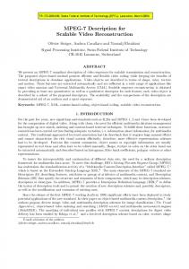
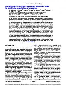
In other words, both δρR and δρL are assumed Gaussian random variables, whose mean values are given by the actual values (respectively, δρa R and δρa L ) and whose variances increase linearly with the travelled distance. Furthermore, it is assumed that δρR and δρL are uncorrelated. With respect to the Chong-Kleeman model, we do not consider systematic errors (i.e. we assumed an odometry system perfectly calibrated). In our simulations, we generated the encoder errors νR/L accordingly to the Gaussian distribution in (22). We set the parameter K = 10−6 m accordingly with the values obtained in previous experiments ([4] and [7]). The data from the encoders are delivered at a frequency equal to 100 Hz. The speed of the robot (vR ) is set equal to 0.2 ms−1 . Regarding the vision sensor we simulated a sensor able to return the bearing angle β in fig. 1 with a Gaussian error. In particular, the variance is assumed to be σβ2 = (1 deg)2 , accordingly with experimental results obtained with an omnidirectional camera [10]. The data from this sensor are delivered at 10 Hz. We set the three parameters characterizing the robot vision sensor reference transformation equal to the following values: φ = ψ = 30 deg and ρ = 0.1 m. We simulated two kind of robot trajectories. In both cases the initial robot configuration is [2, 0, π/2]T and the source of light is at the origin. The first kind of trajectory is random and one example is shown in fig. 2a. In this case the robot moves for 1000s. Each dt = 0.01s the robot is moved by generating randomly the translation of the right and the left wheel. In particular, each translation is generated as a random value, whose mean value is equal to vR × dt and whose variance is equal to 0.01 × vR × dt. Furthermore, the distance between the wheel is set equal to 0.25 m. The second trajectory is shown in fig. 3a. This trajectory consists of pure rotations and pure translations. The length of each segment is about 1 m while each rotation is approximately 450 deg. The robot moves for 100s. Fig. 2b, 2c and 2d refer to the trajectory shown in fig. 2a. They show the results obtained by implementing the EKF introduced in section III to estimate respectively ρ, φ and ψ. The filter is initialized by setting the following values for the three parameters: φ = ψ = 0 deg and ρ = 0 m. It is possible to see that all the parameters converge to the actual values. However, the error is still of the order of 2 deg for the two angles and 1 cm for ρ after 200m of navigation. We obtained similar results by moving the robot along other random trajectories. Fig. 3b, 3c and 3d refer to the trajectory shown in fig. 3a. In this case the convergence is much faster. In particular, only after 4m of navigation, the error is of the order of 0.1 deg for the two angles and 0.1 cm for ρ. We performed many simulations and we found that by moving the robot along this trajectory, the convergence is much faster than by using other trajectories. We remark that this trajectory is not only much more preferable with respect to the other ones because of the fast convergence, but it is also experimentally feasible

a

b

a

b

c

d

c

d

Fig. 2. Results obtained by implementing the strategy introduced in sect. III to estimate the three parameters ρ (fig. b), φ (fig. c) and ψ (fig. d). The considered robot trajectory is displayed in fig. a.

Fig. 3. Results obtained by implementing the strategy introduced in sect. III to estimate the three parameters ρ (fig. b), φ (fig. c) and ψ (fig. d). The considered robot trajectory is displayed in fig. a. At each vertex the robot performs a pure rotation of approximately 450 deg

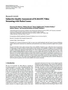
because the robot navigates close enough to the source of light making easy its detection with high accuracy [10]. B. Real Experiments For the experiments we adopted a mobile robot with a differential drive system equipped with encoder sensors on the wheels. We equipped the robot with an omnidirectional vision sensor consisting of a webcam and a conic mirror (see fig 4a). Furthermore, we put on the origin a source of light consisting of a set of LEDs as shown in fig. 4b. Finally, we adopted the same strategy recently introduced in [10] to detect the source of light from the image based on the defocusing. The source of light appears as shown in fig. 4c. We set our sensor on the robot with the following settings: φ  −π, ρ  0.07m and ψ  − π2 , all of them we measured manually. Then, the encoder data and bearing measurements were fused according to the calibration procedure above. The values of the three parameters estimated during motion are plotted versus distance in fig. 5. It is possible to see that after 3 meters of navigation they start to converge to a stable value. Finally, the estimated parameters were φ = −3.11rad, ρ = 0.074m and ψ = −1.58rad. Note that they are consistent with the values measured manually. Also, observe in 5 that the plot of ρ starts at 0 since we took the robot origin as the initial value in the EKF. Nevertheless, its estimation converges to the expected value.

a

b

c

Fig. 4. The conic mirror placed above the webcam (a). The circular set of LEDs forming the light source, positioned at the origin (b). The light source used in our experiments as seen through the adopted vision sensor after defocusing (c): it looks like an ellipse.

VI. C ONCLUSIONS We developed a simple strategy based on the Extended Kalman Filter to estimate the extrinsic parameters of a vision system on a mobile robot. Its implementation only requires a source of light in the environment and an odometry system

47

Fig. 5. The estimated φ, ρ and ψ during the robot motion, plotted vs distance. The adopted units are in this case radians and meters.

on the robot. Furthermore, the estimation is performed automatically during the robot motion. The same strategy can be adopted to calibrate any robot bearing sensor. The strategy was deeply validated through a theoretical analysis. In particular, an observability analysis which takes into account the system nonlinearities was carried out and clearly shows that the system contains all the necessary information to estimate the extrinsic vision sensor parameters. Furthermore, many accurate simulations and experiments performed with real platforms and an omnidirectional conic sensor, fully validated this strategy. In particular, they show that by choosing suitable trajectories, it is possible to estimate the parameters with very high accuracy by moving the robot along very short path (few meters). In the future, we will focus our research on the following topics: • apply optimal control methods in order to find the best robot trajectory which minimizes the error on the estimated parameters; • consider the effect of a systematic component on the odometry; • in the case of an omnidirectional mirror camera, introduce two new parameters (two angles) in order to take into account the orientation of the mirror axis (here assumed aligned with the camera’s optical axis). Acknowledgments This work has been supported by the European project RECSYS (Real-Time Embedded Control of Mobile Systems with Distributed Sensing) and by the Swiss National Science Foundation No. 200021 − 101886.

[11] Zhengyou Zhang. A Flexible New Technique for Camera Calibration, IEEE Transactions on Pattern Analysis and Machine Intelligence, Volume 22, Issue 11, pp.: 1330 1334. November 2000.

A PPENDIX

We want to show that the gradients dL0 β, dL1f1 β, dL1f2 β, dL2f1 f2 β and dL2f2 f2 β are independent. f1 , f2 and β are defined by the equations (21) and (8). We start our proof by computing the five Lie derivatives L0 β, 1 Lf1 β, L1f2 β, L2f1 f2 β and L2f2 f2 β. L0 β = β L1f1 β =

48

a −ρsinφ + Dsinθ ≡ γ γ

(A.2)

b Dρcosθ + D2 ≡ γ γ

(A.3)

L1f2 β =

L2f1 f2 β = 2

2

(A.4)

2

2

Dcosθ(D + ρ ) − 2ρ Dsinθsinφ + 2ρD cosφ c ≡ γ2 γ Dρsinθ(D2 − ρ2 ) d ≡ γ2 γ

L2f2 f2 β =

(A.5)

where γ = D2 + ρ2 + 2ρDcosθ. To prove that the gradients of the previous functions are independent we show that the determinant of the matrix whose rows are these gradients is different from zero. First of all, we remark that only L0 β depends on ψ (see equation (8)). Therefore this matrix has the following structure:

⎡ ⎢ ⎢ ⎣

R EFERENCES [1] Y.Bar-Shalom, T.E.Fortmann,, “Tracking and data association, mathematics in science and engineering”, Vol 179, Academic Press, New York, 1988. [2] Bicchi A., Pratichizzo D., Marigo A. and Balestrino A., On the Observability of Mobile Vehicles Localization, IEEE Mediterranean Conference on Control and Systems, 1998 [3] Bonnifait P. and Garcia G., Design and Experimental Validation of an Odometric and Goniometric Localization System for Outdoor Robot Vehicles, IEEE Transaction On Robotics and Automation, Vol 14, No 4, August 1998 [4] Chong K.S., Kleeman L., “Accurate Odometry and Error Modelling for a Mobile Robot,” International Conference on Robotics and Automation, vol. 4, pp. 2783–2788, 1997. [5] Hermann R. and Krener A.J., 1977, Nonlinear Controllability and Observability, IEEE Transaction On Automatic Control, AC-22(5): 728740 [6] Isidori A., Nonlinear Control Systems, 3rd ed., Springer Verlag, 1995. [7] Martinelli A, Tomatis N, Tapus A. and Siegwart R., “Simultaneous Localization and Odometry Calibration” International Conference on Inteligent Robot and Systems (IROS03) Las Vegas, USA [8] Q.-T. Luong and O. Faugeras, ”Self-calibration of a moving camera from point correspondences and fundamental matrices”, The International Journal of Computer Vision, 22(3):261289, 1997. [9] R. Y. Tsai, ”A versatile camera calibration technique for high-accuracy 3D machine vision metrology using off-the-shelf tv cameras and lenses”, IEEE Journal of Robotics and Automation, 3(4):323344, Aug. 1987. [10] Scaramuzza D., Martinelli A. and Siegwart R., “Precise Bearing Angle Measurement Based on Omnidirectional Conic Sensor and Defocusing”, Proceedings of European Conference on Mobile Robots, ECM R05, Ancona, Italy, September 2005.

(A.1)

∗ ∗ ∗ ∗ ∗

∗ ∗ ∗ ∗ ∗

∗ ∗ ∗ ∗ ∗

∗ ∗ ∗ ∗ ∗

⎤

−1 0 ⎥ 0 ⎥ ⎦ 0 0

Hence, we have to prove that the bottom left submatrix 4 × 4 has the determinant different from zero. In other words, we can consider only the gradients of the last four functions with respect to D θ φ and ρ. Now let us define the following two vectors: − → w = [a, b, c, d]T

− → v = [a, b, 2c, 2d]T

Since γ = 0, the determinant of the previous submatrix is different from zero if and only if is different from zero the following determinant:

  

det = → w ∂− ∂D

−

→ ∂γ − v ∂D γ

→ ∂− w ∂θ

−

→ ∂γ − v ∂θ γ

→ ∂− w ∂φ

(A.6) −

→ ∂γ − v ∂φ γ

→ ∂− w ∂ρ

−

→ ∂γ − v ∂ρ γ

  

On the other hand, through a direct computation it is possible to prove that

  

→ w, ∂− ∂D

→ w, ∂− ∂θ

→ w, ∂− ∂φ

→ w ∂− ∂ρ

   = 0

→ and therefore it is possible to express the vector − v as a combi→ − → → → w , ∂− w , ∂− w and ∂ − w. nation of the four vectors: ∂∂D ∂θ ∂φ ∂ρ → By using this combination for − v in (A.6) it is possible to show that also the determinant in (A.6) is different from zero.