Automatic Software Interference Detection in Parallel Applications Vahid Tabatabaee
Dept. of Computer Science University of Maryland at College Park
[email protected]
ABSTRACT We present an automated software interference detection methodology for Single Program, Multiple Data (SPMD) parallel applications. Interference comes from the system and unexpected processes. If not detected and corrected such interference may result in performance degradation. Our goal is to provide a reliable metric for software interference that can be used in soft-failure protection and recovery systems. A unique feature of our algorithm is that we measure the relative timing of application events (i.e. time between MPI calls) rather than system level events such as CPU utilization. This approach lets our system automatically accommodate natural variations in an application’s utilization of resources. We use performance irregularities and degradation as signs of software interference. However, instead of relying on temporal changes in performance, our system detects spatial performance degradation across multiple processors. We also include a case study that demonstrates our technique’s effectiveness, resilience and robustness.
1.
INTRODUCTION
High-performance computing systems with thousands of processors are used to run large-scale scientific applications. Management and maintenance of such systems are daunting tasks, and it is crucial to have automated supporting tools to help identify problems. In this paper, we present an automated mechanism for software interference and resource contention detection. Performance of parallel applications depends on the combination of user-level application code plus any interfering system level operations. Hence, interfering OS activities can cause resource contention and performance degradation [19,23]. Our objective is to detect and quantify performance irregularities and degradation on individual processors running a parallel application and use the information as an indicator and metric for the intensity of system level interference. Such a metric has several applications in autonomous
Permission to make digital or hard copies of all or part of this work for personal or classroom use is granted without fee provided that copies are not made or distributed for profit or commercial advantage, and that copies bear this notice and the full citation on the first page. To copy otherwise, to republish, to post on servers or to redistribute to lists, requires prior specific permission and/or a fee. SC07 November 10-16, 2007, Reno, Nevada, USA ˇ (c) 2007 ACM 978-1-59593-764-3/07/0011E$5.00
Jeffrey K. Hollingsworth
Dept. of Computer Science University of Maryland at College Park
[email protected]
maintenance and management of high-performance computing systems to detect problems such as: Inconsistent system library and OS kernel setup may cause performance degradation in systems. In large systems with thousands of nodes, it is possible that a system manager fails to update all nodes kernels properly. If such a kernel inconsistency results in performance degradation on some of the cluster nodes, our algorithm could detect it. System software failure is often preceded by performance degradation. Failure prediction systems generally rely on machine learning and statistical inference algorithms to predict failures before they occur. These systems require a local mechanism that can monitor degradation of a node attribute over time. Modern hardware devices are equipped with such monitoring mechanisms. For instance, most disk drives follow the SMART protocol, and provide indication of suspicious behaviors. Similarly, motherboards contain temperature sensors, which can be accessed via interfaces. Network drivers, such as those for Myrinet interface cards, maintain statistics of packet loss and retransmission counts. However, there is no failure detection mechanism for system software. This is despite the fact that most failures are due to software errors. For instance, failure logs for an eight-month period from the Platinum and Titan clusters at NCSA shows that while 0.1 and 5 percent of failures were due to hardware errors, 84 and 60 percent of them were due to software errors respectively [8]. Our proposed mechanism can be used as a failure detection and monitoring mechanism for early prediction of software errors. Software aging is a phenomenon, usually caused by resource contention that can cause computer systems to hang, panic, or suffer performance degradation. Software rejuvenation is a proactive fault management technique for cleaning up the system and for preventing severe failures or systems performance degradation. Proactive rejuvenation (sometimes called therapeutic reboots) can include re-initialization of components, purging shared-memory buffer pool caches, or node fail-over. In a prediction-based rejuvenation system, our proposed mechanism can be used to activate the rejuvenation mechanism(s) to avert catastrophic failures. Previously, the general approach for failure prediction and interference detection has been to monitor and collect information on critical resource attributes such as CPU, disk, memory and network. Then, by using statistical, machine learning and curve fitting techniques try to predict and detect software interference or failure [1, 5, 6, 15]. For every fixed configuration, this approach requires multiple sampling of the normal system behavior to tune its detection param-
eters. In our approach, instead of system resource utilization, we first monitor the short term performance of the application. Then, we compare every processor’s performance with a base line formed from the average and standard deviation of all processors’ performance. Hence, instead of relying on absolute performance measurements of each processor separately, we consider the relative performance of processors to detect performance degradation of individual processors. If the relative performance of the processors does not vary dramatically for different configurations, previously collected performance data may be re-used to detect anomalies in later runs. Further, instead of direct and explicit comparison of processors performance, we first use the MPI profiles to detect common patterns in the processor profiles. Then, we compare performance of the processors during the execution of these common patterns. In this way, our approach can also work for irregular and unbalanced applications, as long as there are some common patterns in the processor profiles. Solution Overview: Our goal is to develop general interference monitoring algorithms for MPI applications. For each processor we form a 4-tuplet profile sequence. The first entry is the MPI function, the second one specifies the corresponding peer processor(s) of the MPI call, the third entry is the time elapsed since the last MPI call (computation time) and the fourth entry is the elapsed time in this MPI call (communication time). We abstract the sequence of the first two tuplets to a grammar that describes the behavior patterns. This abstraction enables us to extract Typical Sequences (TS) that are common patterns of inter-processor interaction. After identifying an application’s typical sequences, we monitor the computation (communication) time of typical sequence occurrences for all processors. For each processor and typical sequence we have a time series. Further, for each typical sequence we aggregate data from all processors to form two additional time series, whose values are the average and standard deviation of the individual processor samples for that sequence. Processor typical sequence samples are compared against dynamic threshold values computed from the average and standard deviation data. We form an Interference Level Signal (ILS), which is the running average of the number of processor samples that are above their corresponding threshold value. Finally, for each processor, we combine all typical sequences interference level signals to compute the interference metric, a positive number whose value indicates interference level for the program running on that processor. Dynamic threshold values are computed separately for each processor and typical sequence, even though all of them are functions of the same average and standard deviation. Therefore, what we measure is the relative deviation of performance with respect to the average and standard deviation rather than absolute performance values. Hence, our approach is resilient to natural temporal performance variations as long as the relative performance does not change dramatically. Our main contributions in this paper are: 1. We use MPI1 profiling to monitor and separate com1
Even though we have used MPI profiling in our current implementation of the algorithm, similar methodology would work with other parallel programming languages such as
putation and communication components of the performance. 2. We use the Sequitur algorithm [22] to automatically extract typical repeated communication sequences that are common to all processors. 3. Our approach takes advantage of the spatial and relative performance correlation between processors that frequently exists in SPMD parallel applications. The rest of the paper is structured as follows: In section 2, we briefly review MPI profiling and the Sequitur algorithm. In section 3, we go over the main challenges in the design of our algorithms to provide the rationale for our proposed solutions. In section 4, we introduce the main components of our proposed algorithm. In section 5, we study performance and characteristics of the algorithm on the NAS [2] benchmarks and a production level scientific application called Parallel Ocean Program (POP) [25]. In section 6, we review and discuss related work.
2. 2.1
PRELIMINARIES AND TOOLS MPI Profiling
We use the MPI profiling interface to perform our data gathering. The idea behind the MPI profiling interface is to use the linker to substitute a user-written wrapper function for the MPI functions called by the application. Every MPI function with the name MPI Xxx is also callable by the name PMPI Xxx name. Hence, we write a wrapper function with the same name MPI Xxx, where we do profiling as well as calling the real MPI function by the name PMPI Xxx. At the start and end point of wrapper functions, we save the wall time value. The computation time for an MPI call is the difference between the current MPI call starting time and the previous MPI call ending time. We also save the wall time values before and after calling the real MPI function inside the wrapper. The difference between these two values is the communication time of the current MPI call.2 For each MPI call, we also record the peer processor. For instance, the peer processor for an MPI send is the destination processor. For those collective operations that do not have an explicit peer processor, we select an appropriate parameter or set it to a fixed number based on the collective operation. For instance, for MPI Reduce, we use the operation indicator parameter (i.e. MPI Sum), for MPI Wait we use a constant value and for MPI Barrier we use the communication group. The profiling data for each MPI function call is a 4-tuplet consisting of the MPI function name, peer processor, computation and communication time. The profiling information is monitored and saved for each processor separately.
2.2
Abstracting MPI event logs
After generating MPI profiles, we focus on the first two entries (MPI function and peer process) to find repeated patterns. From these patterns, we extract typical sequences OpenMP, UPC and Titanium. 2 We assume that there is at most one application process per processor, so the wall time is a good proxy for communication time.
Table 1: Example sequences and Sequitur grammars that reproduce them Sequence
Grammar
S→abcdbc
S→aAdA A→ bc
S→abcdbcabcdbc
S→AA A→ aBdB B→ bc
(a) (b)
that are common among all (or a subset of) processor profiles, and hence their computation time are relatively comparable. Simple programs often have a semi-periodic pattern that can be easily detected. We can detect these patterns by simple signal processing techniques that are based on using the auto-correlation function of the profile sequence. In complex applications, common patterns still exists but they may not be periodic, hence we can not rely on simple signal processing algorithms to detect them. Instead, we use the Sequitur algorithm to extract the frequent patterns. The Sequitur algorithm is a linear-time, online algorithm for producing a context-free grammar from an input string [22]. Sequitur takes a sequence of discrete symbols, which in our case represents the MPI function and peer process in the profile sequence, and produces a set of hierarchical rules as a context-free grammar. Note that there is no generalization in the produced grammar and it can only generate one string, which is the original sequence. Sequitur produces a grammar based on repeated phrases (patterns) in the input sequence. Each repetition gives rise to a rule in the grammar. Hence, there are high frequency patterns among the rules derived. At each step, Sequitur appends a new symbol from the input sequence to the end of the produced grammar up to that time. After adding each symbol, Sequitur modifies the grammar to maintain two properties: 1-Diagram Uniqueness: no pair of adjacent symbols appears more than once in the grammar. 2-Rule Utility: every rule is used more than once. Table 1 shows simple examples (adopted from [22]) of the inputs and outputs to the algorithm. The original sequence symbols and Sequitur generated rules are shown with lowercase and capital letters respectively. Rule S generates the whole sequence. In example (a) Rule A corresponds to the pattern bc, which is repeated two times in the original sequence. In example (b), we have appended 6 new letters to the example (a) sequence. Sequitur forms A and B rules, whose corresponding sequences are abcdbc and bc respectively.
3.
REQUIREMENTS, CHALLENGES AND SOLUTIONS
We now elaborate on some of the problems and challenges in the design of interference detection algorithms. We present these issues to explain the reasoning behind the design of our interference detection algorithm. Insensitivity to the network performance: Communication and computation times determine the overall performance of parallel applications. While software interference increases the computation time, it is not clear how it affects the com-
munication time. Software interference may change when a processor’s data is ready and/or when it needs new data. This in turn changes the communication pattern between processors and consequently can remove or create network bottlenecks and hence reduce or increase the communication time. Therefore, it is crucial to monitor and profile the communication and computation times separately. Appropriate time scale: In our approach, we monitor software performance to estimate software interference levels. However, software interference is not the sole cause of performance variations and we need to minimize other factors too. Kernel scheduler granularity is another reason for performance variation. Consider that under normal behavior it might be the case that 99 percent of the processing time is allocated to the application and 1 percent is consumed by the OS and daemon processes. Suppose that the kernel scheduler granularity is 5ms. Roughly speaking, the processor spends 495ms (99 × 5) running the application and 5ms running other things. If the monitored computation time granulaity is close to the kernel scheduler granularity (5ms), even under normal operation, we will observe significant variations. In general, the impact of factors other than interference becomes evident and more significant for smaller computation times. This is because while the absolute value of performance variations remain the same, for smaller intervals of time their relative impact is higher.3 To reduce sensitivity to normal performance variations, we use aggregation and filtering. To increase the time duration of samples, instead of considering individual samples, we work with the aggregated patterns derived by Sequitur. Further, we drop computation time intervals that are lower than a pre-defined threshold. The threshold value is not fixed and we will discuss in section 4.3 how it is set. Another major source of performance variation is the application itself. It is quite possible that between different occurrences of the same MPI profile pattern, the application runs a different set of instructions which results in temporal variations in the monitored performance. Hence, instead of temporal, we use spatial correlations in our analysis. Note that, we do not require that application performance on all processors be the same, or even they execute same instruction sequence. As long as, there are some common communication patterns among some processors and their relative performance does not change dramatically our algorithm performs well. Insensitivity to Software Configuration: Software performance may depend on an application’s compile and/or run time parameters. This is problematic for interference detection algorithms that are based on statistical and machine learning approaches and rely on similarities in temporal performance patterns. Note that for each new software configuration, these algorithms need to learn the temporal patterns again. The number of possible configurations can be very large, which makes it practically impossible to train the detection algorithm for all possible configurations. By using relative spatial rather than absolute temporal performance correlation, our algorithm is less sensitive to software configuration variations. In other words, we assume the detected communication patterns that occur frequently in the profile remain frequent from run to run, while the timing and 3
While some applications might be subject to performance degradation due to these small changes in system overhead, we concentrate on identifying larger gained interference.
repetitions count of the patterns may change.
4.
THE ALGORITHM
In this section, we present the main modules of the detection system and explain how they interact with each other. The input to the system are processor profiles that contain application MPI calls, peer process, computation time and communication time as explained in section 2. Further, we use the Sequitur algorithm to form the frequent patterns for only one of the processors. We divide the system into three main modules which are: preprocessing, learning and detection units.
4.1
Preprocessing Unit
The preprocessing unit generates signals that are inputs to other units. First, we need to select a subset of the Sequitur patterns that are frequently present in all processor profiles. To that end, we sort the Sequitur patterns according to their length. We start from the longest pattern and determine how many matches we find in each processor’s profile sequence. To find a match, we only check the first entry in the profile, i.e. the MPI function. Recall that the Sequitur patterns are generated based on the MPI functions and peer processor entries in a processor profile. However, since the peer processor entry is processor dependent, we can not use it at this stage to find matches among different processors. We select the first L Sequitur patterns that were detected frequently on all processors and call them the Typical Sequences (TS). For each TS, we form P processor signals, where P is the number of processors. For a given processor p and a typical sequence l, the processor signal consists of the computation time of typical sequence l’s occurences for processor p. We also form two aggregate signals that represent the average and STD. deviation of all processor samples. Note that average and standard deviation are taken over all processors signals at each sample index. Therefore, we have L × (P + 2) signals. We denote by S(p, l, t) the computation time of the t-th occurence of typical sequence l on processor p. We define AV G(l, t), ST DEV (l, t) the average and standard deviation signals, PP AV G(l, t) = P1 p=1 S(p, l, t) q ST DEV (l, t) =
4.2
1 P
PP
(1)
2 p=1 (S(p, l, t) − AV G(l, t))
Detection Unit
The outputs of this unit are interference level signals and interference metrics. For each processor and TS we compute a dynamic threshold, T (p, l, t) = AV G(l, t) + K(p, l) × ST DEV (l, t),
(2)
where K(p, l) is a constant determined in the learning unit. Whenever a signal sample is above the corresponding threshold, the contention level assessment should be increased. The indicator function I(p, l, t) specifies when a signal is above that threshold: ½ 1 if S(p, l, t) > T (p, l, t) I(p, l, t) = (3) 0 if S(p, l, t) ≤ T (p, l, t) In section 3, we elaborated on the sensitivity to normal variations in application performance, and mentioned that we
filter out samples that are for too short of time intervals. We filter signal samples that are less than 0.5ms. We take the running averages of the filtered indicator functions and call them the Interference Level Signal (ILS(p, l, t)). Hence, ILS(p, l, t0 ) is the average of those indicator function samples [I(p, l, 1) · · · I(p, l, t0 )], whose corresponding S(p, l, t) intervals are longer than 0.5ms. Interference increases both the signal level S(p, l, t), and the number of times that it is larger than the threshold T (p, l, t). Consequently, this results in a larger average value, i.e., the interference level signal ILS(p, l, t) is larger. We use the interference level signals to derive a single interference metric, m(p). In this paper, we use a weighted average of the signals final values: X m(p) = w(l)ILS(p, l, end), (4) l
where the weight w(l) of typical sequences is proportional to sequence length. As we will see in the case study longer typical sequences are more stable and less sensitive to normal performance variations, hence we give them higher weights in the metric computation. Clearly there are alternative ways to define this metric. For instance, we could take a maximum instead of an average over all typical sequences, or instead of the last value, we could use maximum or average of all values. We will consider and compare alternative options in the future. We note that the Detection unit tasks can be done in real time as the program is running. Since we are taking the average and standard deviation of computation time samples and using a running average of the (filtered) indicator function, we do not need any future information to compute the value of the metric at time t. The interference metric is also defined over time as the weighted average of the last computed ILS signals. In the next section, we specify how we compute K(p, l) during the learning phase.
4.3
Learning Unit
Learning is performed once per application prior to production runs to select and tune the detection algorithm parameters. The objective of this step is to set K(p, l). To that end, for each processor we gather two sets of signals. The first set is for a normal run of the application without any background activity. In the second set, we run a simple background interfering job on the node. To quantify the impact interference, we want to set the parameters K(p, l) so that we have as much difference as possible in the interference level signal final values of the two runs. After generating the S(p, l, t), AV G(l, t), ST DEV (l, t) signals for the two runs, we compute alternative threshold functions by using different values of k, k = 0, 0.5, · · · , 10 for K(p, l) in (2). Then, we compute the indicator functions defined in (3) for different threshold functions. Let ILSN or (p, l, end, k) and ILSInt (p, l, end, k) be the final value of the indicator level signals of the two runs (without and with background loads respectively). Note that these values are a function of the parameter k. Then we select the threshold value that maximizes the difference: ³ ´ k k (p, l, end) − IN (5) K(p, l) = arg max IInt or (p, l, end) k
If for a processor p and a typical sequence l, and for all values of k the resulting value is small, we do not use the typical sequence l in the detection unit of processor p. This
Table 2:
Length of FT MPI Profile Typical Sequences 1
2
3
4
FT-F-1
FT-O-1
FT-N-1
length
16
8
4
2
0.324
0.1284
0
PERFORMANCE EVALUATION
In this section, we evaluate and study the performance of the proposed interference detection algorithm for 3 parallel bechmarks and applications. We run each application without interfering jobs, with a continuously interfering back ground job on a single node and with an on-off interfering job on a single node. The on-off job runs for approximately 10 seconds and then becomes idle (sleeps) for 5 seconds. We ran all applications on 64 processors (32 nodes) of a Linux cluster. Each node is equipped with dual Intel Xeon 2.66 GHz processors. Nodes are connected via Myrinet network, and use the PBS batch scheduler to admit at most one application per node at a time. To run the application and the interfering job simultaneously, we reserved nodes in interactive mode, so we could login to a desired node and run the background job while we were running the parallel application. For our experiments hyperthreading was turned off, and each processor of a node runs a separate task of the application to make sure there is exactly one application process per processor.
5.1
NAS Benchmarks
In this section, we evaluate the performance of our system for interference detection on FT and CG, which are two of the NAS parallel kernels derived from computational fluid dynamics applications. The NAS parallel benchmarks (NPB) [2] were developed at the NASA Ames research center to evaluate the performance of parallel and distributed systems.
5.1.1
Interference Metrics for FT runs
TS
step eliminates typical sequences that are not sensitive to interference.
5.
Table 3:
FT Benchmark
The NAS FT benchmark is a three-dimensional heat equation solver that solves a certain partial differential equation using forward and inverse FFTs. This kernel performs the essence of many spectral codes. It is a rigorous test for longdistance communication performance. We run FT class C on 64 processors (32 nodes). The structure of the FT MPI profile is very simple. It consists of 47 MPI calls and after a few initializing calls it periodically calls MPI Alltoall and MPI Reduce functions. From the Sequitur grammar we get 4 sequences, whose length are given in table 2. The typical sequences are in fact 1, 2, 4 and 8 repetitions of the pattern (MPI Alltoall, MPI Reduce). Even though the output pattern is very simple, this experiment confirms that Sequitur can detect highly regular periodic patterns. We examined the performance of the interference detection algorithm on node 1. We first use two runs with a continuous (full) and no background jobs for the learning phase. Figure 1 shows the ILS(p, l, t) for p = 1, 2 and l = 1, · · · 4 signals for two production (non-learning) runs. One of the two runs is with continuous (full) background (FT-F-1) job and the other one is with no background job (FT-N-1). In
all ILS plots, the x-axis is TS sample index t and y-axis is the interference signal level. In the figure, we can only see the ILS signal for the run with background (the red plot), since the ILS signal for the run with no background job remains zero and thus lies on the x-axis. Hence, as expected, the ILS signal is positive when there is interference and is zero when there is no interference. We can also see that when there is a background job, the ILS signal associated with longer typical sequences are larger, and hence they are better detectors. This is due to the fact that for longer sequences, we aggregate a larger number of MPI profile samples and thus lessen the sensitivity to natural temporal performance variations. Figure 2 shows the ILS signals for two processors with on-off (FT-O-1) and no background jobs. The ILS signals for the on-off background job are positive and for without the background job are zero. Signal levels in figure 2(a) are smaller than the signal levels in figure 1(a) indicating lower interference levels. Table 3 summarizes the FT runs interference metrics as defined in (4). These results confirm the positive relation between the interference level experienced by the application and our metric. We now study the sensitivity of our interference metric to variations in the on-off period of background jobs. Table 4 shows our interference metric for different combinations of on and off periods of the background job. Our metric is able to detect interference for all of these cases (i.e. we get nonzero values for the metric). However, when the background job active (on) time period is 1s and its inactive (off) time period is larger than 20s the metric gets close to zero. In some cases, even though the metric correctly detects the interference, its value does not accurately represent intensity of the background job. To understand the reason behind this fluctuation of the interference metric, we need to elaborate more on the pattern of computation in FT. In FT, all processors regularly exchange data with each other, which results in significant communication time. In our experiments the FT program spends about twice as much time performing communication as computation. Note that if the background job uses CPU only during FT’s communication periods, there will be no interference. Therefore, the interference metric value depends on: (1) the intensity of the background jobs, and (2) the duration of the over-lap between the on-periods of the background job and the computation period of the FT program. The first factor is deterministic, but the second one is in general probabilistic. That is why we observe fluctuations in the performance metric value. In our experiments, a complete run of FT takes about 2 minutes. Now, consider the case where the background job’s active period is 1 second (third row) and its in-active period is 20 seconds (5th column). There are approximately 6 onperiods of the background job during a complete run of FT. The interference metric value depends on the overlap time between the 6 active periods of the background job and FT’s computation times (which are about 40 seconds out of the
1
1.5
0
2
2
3
4
5
1
0.5
0
2
4
6
ILS(2, 2, t) 1
1.5
1
0.5
2
4
6
t
8
1
0.5
2
4
t
2
3
4
5
6
6
1
0.5
0
8
2
4
6
t
(a) Processor 1 Figure 1:
1
1.5
0
10
1
0.5
0
2
1.5
0
8
1
0.5
0
6
1.5
ILS(1, 4, t)
ILS(1, 3, t)
1.5
1
ILS(2, 3, t)
0
1
0.5
1.5
ILS(2, 4, t)
1
0.5
1.5
ILS(2, 1, t)
1.5
ILS(1, 2, t)
ILS(1, 1, t)
1.5
8
10
t
(b) Processor 2
ILS(p, l, t) vs t plots for FT kernel with full, and no background jobs for p = 1, 2 and l = 1, · · · , 4. The plots for the
run with background are shown with red lines, but the plots for the run with no back-ground are always zero and lie on the x-axis.
1
1.5
0
2
2
3
4
5
1
0.5
0
2
4
6
1
2
4
6
t
8
10
t
ILS(2, 2, t) 1.5
0
2
1
2
3
4
5
6
1.5
1
0.5
0
1
0.5
2
4
6
8
1
0.5
0
2
t
(a) Processor 1 Figure 2:
1
1.5
0.5
0
8
1
0.5
0
6
1.5
ILS(1, 4, t)
ILS(1, 3, t)
1.5
1
ILS(2, 3, t)
0
1
0.5
1.5
ILS(2, 4, t)
1
0.5
1.5
ILS(2, 1, t)
1.5
ILS(1, 2, t)
ILS(1, 1, t)
1.5
4
6
8
10
t
(b) Processor 2
ILS(p, l, t) vs t plots for FT kernel with on-off, and no background jobs for p = 1, 2 and l = 1, · · · , 4. The plots for
the run with on-off background are shown with red lines, but the plots for the run with no back-ground are always zero and lie on the x-axis.
Table 4:
Interference Metrics for FT with different On-Off
times Off time(s) 15 20
On time(s)
5
8
10
10 3 1
0.63 0.69 0.58
0.57 0.50 0.30
0.84 0.44 0.10
Table 5: TS length
0.58 0.53 0.07
0.89 0.32 0.09
25
30
0.7 0.36 0.03
0.52 0.32 0.03
Length of CG MPI Profile Typical Sequences
1
2
3
4
5
6
7
8
25428
12624
6312
3156
1578
789
720
480
120 seconds of FT’s run time). The overlap time is clearly a random variable, and hence the reason behind the fluctuation of the results. Therefore, the most important factor is not duty cycle of background jobs, but the probability of overlap (interference) between the computation time and interference.
5.1.2
CG Benchmark
The CG benchmark uses the inverse power method to estimate the largest eigenvalue of a symmetric positive definite sparse matrix with a random pattern of non-zeros. This
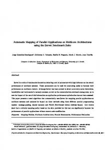
kernel is typical of unstructured grid computations in that it tests irregular long distance communication, employing unstructured matrix vector multiplication. The MPI profile of CG is much more complex than FT. We ran CG class C on 64 processors (32 nodes) and the profiles contain around 60,000 MPI calls. Sequitur generates 23 rules (patterns) and we selected the 8 longest ones as the typical sequences. Their lengths are given in table 5. Figure 3 shows the autocorrelation function of the MPI profile integer representation. The auto-correlation of periodic signals are periodic and their maximums are at 0 and multiples of the period. In fact, auto-correlation is commonly used to find the period of periodic and semi-periodic patterns in a signal. The autocorrelation function in figure 3 indicates the presence of two periodic components. The first one repeats every 30 sample and the second one repeats after 789 samples as shown on the figure. The first six typical sequences are repetitions of the 789 samples pattern and the last two ones are repetitions of the 30 sample pattern. Hence, even in complex situations, where multiple semi-periodic patterns coexist, Sequitur successfully detects them. After using two runs for learning, we use two separate runs for evaluation of the system. Figure 4 shows the ILS signals for two processors with continuous (CG-F-1) and no background job (CG-N-1) runs. The ILS signals for the no background runs are always zero, and hence not visible on the plot. It is also clear that the ILS signals of longer typical sequences are larger and hence more reliable for interference
Autocorrelation function for CG MPI encoded samples 21.5 peaks repeat every 789 samples
21
20.5
peaks repeat every 30 samples
20
19.5
19
18.5
18
17.5
100
ILS(1,5,t)
ILS(1,4,t) 0
0.5
1 1.5 Sample Count
0.5 0
0.5
1 1.5 Sample Count
ILS(1,7,t) 0
0
0.5
1 t
x 10
1.5
2
2 4
x 10
0
0.5
1 1.5 Sample Count
0.5 0
0.5
1.5
1 1.5 Sample Count
x 10
1 0.5 0
0
0.5
4
x 10
1 t
1.5
0.5 4000
6000
8000
10000
0
0.5
1
1.5
1.5 1 0.5 0
0.5
1
1.5
1.5
x 10
1 0.5 0
4
x 10
0.5
1 t
1.5
2
0.5
1
1.5
2 4
x 10
1 0.5 0
0.5
1
1.5
1.5
2 4
x 10
1 0.5 0
2 4
0
1.5
0
2 4
x 10
1 0.5 0
12000
0.5
(a) Processor 1 Figure 4:
2000
1
0
2
0
1.5
0
2 4
CG Processor 2 1.5
1
0
2 4
x 10
1
0
2 4
1 1.5 Sample Count
0.5
1.5
800
ILS(2, 2, t)
ILS(2, 1, t)
0.5
1
0
2 4
x 10
1
0.5
0
1.5
700
1.5
0 ILS(2, 3, t)
15000
0.5
1.5
0.5
ILS(2, 5, t)
5000 10000 Sample Count
1
600
Cross-correlation function of MPI encoded profile.
ILS(2, 7, t)
0
1.5
0
500
1
0
ILS(1,6,t)
ILS(1,3,t)
ILS(1,2,t)
0.5
ILS(1,8,t)
ILS(1,1,t)
1
0
400 Shift
CG Processor 1 1.5
1.5
0
300
ILS(2, 4, t)
Figure 3:
200
ILS(2, 6, t)
0
ILS(2, 8, t)
17
0
0.5
1
1.5
1.5
2 4
x 10
1 0.5 0
0
4
x 10
0.5
1 t
1.5
2 4
x 10
(b) Processor 2
ILS(p, l, t) vs t plots for CG kernel with full, and no background jobs for p = 1, 2 and l = 1, · · · , 8 (first run). The
plots for the run with full background are shown with red lines, but the plots for the run with no back-ground are always zero and lie on the x-axis.
Table 6:
Interference Metrics for CG runs
CG-F-1
CG-F-2
CG-O-1
CG-N-1
CG-N-2
0.78
0.77
0.61
0
0
detection. Figure 5 shows the output of the system for two additional runs with the same type of background jobs (CGF-2 and CG-N-2). Even though the output signal is not the same, it has the same characteristics. For example, it is zero for the no background run and longer typical sequences result in larger signals when there is a background job. From the FT and CG results, we may conclude that longer typical sequences are better candidates for interference detection. Figure 6 shows the performance of the algorithm when there are on-off background jobs (CG-O-1). The algorithm can still detect interference but the sensitivity of the shorter typical sequences is higher and they are clearly less reliable. Table 6 summarizes the CG runs interference metrics as defined in (4). The results confirm the relation between the interference level on the node and the computed metric. As expected, the two runs with full background jobs have the greatest interference metric values, followed by the run with on-off background jobs. The metric value is zero for all runs without background job.
5.2
POP Program
The Parallel Ocean Program (POP) [12] was developed at Los Alamos National Laboratory and is descendant of the Bryan-Cox-Semnter class of ocean models first developed at
the NOAA (National Oceanic and Atmospheric Administration) Geophysical Fluid Dynamics Laboratory in Princeton, NJ in the late 1960s [3]. POP is currently used by the Community Climate System Model (CCSM) as the ocean component. The model solves the three-dimensional primitive equations for fluid motions on a sphere using hydrostatic and Boussinesq approximations. Figure 7(a) depicts the profile of the computation time for 4 processors4 . Clearly the processor 1 (top-left) profile is different from other processors, hence it is not possible to detect interference by direct comparison of profiles. Figures 7(b) and 7(c) are the computation time for two typical sequences occurrences on the same 4 processors. The derived patterns for the 4 processors are comparable, and hence we can use spatial correlation to detect interference. Furthermore, due to profile sample aggregation in a single sequence, and elimination of samples that are not in typical sequences, the total number of samples are greatly reduced compare to the full event trace, which results in reduced processing time. We started with Sequitur patterns derived from processor 1 profile. Then, we found 10 typical sequences among them that are also present in other processor profiles whose length was long enough (larger than 50) to be considered. The length of the typical sequences are given in table 7. From each processor profile, we obtain 10 TS derived signals. Eight of the TS derived signals are similar to figure 7(b) and two of them (number 5 and 9) are similar to figure 7(b).
5.2.1 4
Interference on Node 2
We show results for 4 out of 64 processors due to space limit, however all processors follow a similar pattern.
1.5
0
0.5
1
1.5
2 4
x 10
1 0.5 0 1.5
0
0.5
1
1.5
2 4
x 10
1 0.5 0
0
0.5
1 t
1.5
2
0.5
1
1.5
2 4
x 10
0.5 0 1.5
0
0.5
1
1.5
2 4
x 10
1 0.5 0 1.5
0
0.5
1
1.5
2 4
x 10
1 0.5 0
0
0.5
4
x 10
1 t
1.5
2
ILS(2, 2, t)
ILS(2, 1, t) 0
1
0.5 0 1.5
0
5000
10000
1 0.5 0 1.5
0
0.5
1
1.5
2 4
x 10
1 0.5 0 1.5
0
0.5
1
1.5
2 4
x 10
1 0.5 0
0
0.5
4
x 10
1 t
(a) Processor 1 Figure 5:
15000
ILS(2, 4, t)
0.5
1.5
1
ILS(2, 6, t)
15000
0
ILS(2, 3, t)
10000
0.5
Processor 2 1.5
1.5
1.5
ILS(2, 8, t)
ILS(1, 5, t)
5000
1
0
ILS(1, 7, t)
0
ILS(1, 4, t)
1.5
ILS(1, 6, t)
0
ILS(2, 5, t)
0.5
ILS(2, 7, t)
1
ILS(1, 2, t)
Processor 1 1.5
1
ILS(1, 8, t)
ILS(1, 1, t) ILS(1,3,t)
1.5
2
1 0.5 0 1.5
0
0.5
1
1.5
2 4
x 10
1 0.5 0 1.5
0
0.5
1
1.5
2 4
x 10
1 0.5 0 1.5
0
0.5
1
1.5
2 4
x 10
1 0.5 0
0
0.5
4
x 10
1 t
1.5
2 4
x 10
(b) Processor 2
ILS(p, l, t) vs t plots for CG kernel with full, and no background jobs for p = 1, 2 and l = 1, · · · , 8 (second run). The
15000
0.5 0 1.5
0
0.5
1
1.5 x 10
1 0.5 0 1.5
0
0.5
1
1.5
2 4
x 10
1 0.5 0
0
0.5
1 t
1.5
2
0
1
1.5
2 4
x 10
0.5 1.5
0
0.5
1
1.5
2 4
x 10
1 0.5 0 1.5
0
0.5
1
1.5
2 4
x 10
1 0.5 0
0
4
x 10
0.5
1 t
1.5
2 4
x 10
(a) Processor 1 Figure 6:
ILS(2, 2,t)
ILS(2, 1, t) 0.5
1
0
2 4
1.5
0.5 0 1.5
0
5000
10000
15000
t
ILS(2, 4, t)
10000
0
1
1 0.5 0 1.5
0
0.5
1 t
1.5
2 4
x 10
1 0.5 0 1.5
0
0.5
1 t
1.5
2 4
x 10
1 0.5 0
0
0.5
1 t
ILS(2, 6, t)
5000
1
0.5
Processor 2 1.5
1.5
1.5
2
ILS(2, 8, t)
0
ILS(1,4, t)
1.5
ILS(1, 6, t)
0
ILS(2, 3, t)
0.5
ILS(2, 5, t)
1
ILS(2, 7, t)
Processor 1 1.5
1
ILS(1, 2, t)
1.5
ILS(1, 8, t)
ILS(1, 7, t)
ILS(1, 5, t)
ILS(1, 3, t)
ILS(1, 1, t)
plots for the run with full background are shown with red lines, but the plots for the run with no back-ground are always zero and lie on the x-axis.
1 0.5 0 1.5
0
0.5
1 t
1.5
1 t
1.5
1 t
1.5
1 t
1.5
2 4
x 10
1 0.5 0 1.5
0
0.5
2 4
x 10
1 0.5 0 1.5
0
0.5
2 4
x 10
1 0.5 0
0
4
x 10
0.5
2 4
x 10
(b) Processor 2
ILS(p, l, t) vs t plots for CG kernel with on-off, and no background jobs for p = 1, 2 and l = 1, · · · , 8. The plots for the
run with on-off background are shown with red lines, but the plots for the run with no back-ground are always zero and lie on the x-axis.
Here, we introduce interfering jobs on node 2 (processor 3 and 4). We first run POP, once with no background and once with a continuous background job on node 2. We then generate the TS derived signals of the two runs and use them in the learning phase to compute the interference detection system parameters. In the learning phase, if the maximum difference between the ILS signals of the two runs is close to zero then that typical sequence will not be used for detection. For node 2, this occurred for typical sequences 5 and 9. Therefore, we focus and use the remaining 8 sequences for node 2. The discarded sequences are those that show the least sensitivity to interference. For evaluation, we generate two new profiles with full (PPN2-F-1) and without (PPN2-N-1) background jobs on node 2. The POP configuration was similar to the first set used in the learning phase. Figure 8 shows the ILS signals for the two processors (processor 3 and 4) on node 2. The ILS signals for the no background run are always zero, and hence lie on the x-axis. The ILS signals for the run with continuous interference are shown in the plots. For the next set of experiments, we changed the POP configuration to asses our tool’s ability to detect interference when the workload of an application is changed. In particular, we changed the stop count parameter of POP from 40 to 20. We ran the algorithm 3 times with no (PPN2-N-2), continuous (PPN2-F-2) and on-off (PPN2-O-2) background jobs. In the detection unit, we used the threshold values
that were derived using runs with the previous POP configuration. Figure 9 shows the ILS signals for the runs with continuous and without background jobs. Again, the ILS signals for the no background runs remain zero, and hence are not visible on the plot. The result for a continuous background job on processor 3 is also zero. Note that we did not have any control on how the OS kernel schedules the background job on node processors. In this case, the background job was always scheduled on processor 4. Hence, there is no interference on processor 3. This result also indicates that we need to monitor the performance of all processors running on multi-processor/multi-core node simultaneously and compute the performance metric for a node based on the ILS signals of all processors. Figure 10 shows the result for the runs with on-off traffic and without background jobs. The ILS signal for the no background run is always zero and hence lies on the x-axis. Since the background job is on-off and less intense, the interference level is lower than in previous experiments. This is reflected in the ILS signal values. Contrary to the previous case, the interference is detectable on both processors results. This is a by-product of the kernel scheduler, not a characteristic of the application. Table 8 provides the interference metrics for all runs that we discussed in this section. The metric correctly detects runs with interference, since the values for runs with the background job are positive and for runs without the background activity are zero. The metric values of the two runs
Table 7:
Length of the POP MPI Profile Typical Sequences
TS length
1.4
1
2
3
4
5
6
7
8
9
10
252
224
192
128
125
112
96
64
64
56
Typical Sequence 1 Computation Time for POP 0.05
MPI Profile Computation TIme for POP 0.05
0.05
0.04
0.04
0.04
0.8
0.03
0.03
0.03
0.6
1.2
Typical Sequence 5 Computation TIme for POP 0.7
1
0.6 0.5
0.02
0.02
0.01
0.01
0.01
0
0
Time
0.02
Time
Time
0.6
Time
Time (s)
Time (s)
1 0.8
0.4
10
0
4
x 10
5 Sample Index
10
2000
4
x 10
4000 6000 Sample Count
8000
0
10000
0.05
0.05
0.04
0.04
0.04
0.04
0.03
0.03
0.03
0.03 0.02
0.02
Time
0.05
Time
0.05
0.02
0
2000
4000 6000 Sample Count
8000
0
10000
0.02
50
100 150 Sample Count
200
0.01
0.01
0
5 Sample Index
0
10
0
4
x 10
5 Sample Index
10 4
x 10
0.01
0.01
0
0
0
2000
4000 6000 Sample Count
8000
10000
0.7
0.7
0.6
0.6
0.5
0.5
0.4
0.4
0.3
2000
4000 6000 Sample Count
8000
10000
0
0
50
100 150 Sample Count
200
250
0
50
100 150 Sample Count
200
250
0.3 0.2
0.1
0
0
250
0.2
0
0.3
0.1 0
Time
5 Sample Index
Time (s)
Time (s)
0
0
0.2
Time
0.2 0
0.4
0.2
0.4
0.1 0
50
100 150 Sample Count
200
250
0
(a) Pure profile computation time (b) Typical sequence 1 signal samples (c) Typical Sequence 5 signal samples Figure 7:
Table 8:
Pure profile and typical sequence samples computation times for first four processors
Interference Metrics for POP runs with back-
ground activity on node 2. PPN2-F-1
PPN2-F-2
PPN2-O-2
PPN2-N-1
PPN2-N-2
0.086
0.324
0.1284
0
0
Table 9:
Interference Metrics for POP runs with background activity on node 1 PPN1-F-1
PPN1-F-2
PPN1-O-2
PPN1-N-1
PPN1-N-2
0.23
0.25
0.19
0.01
0.01
are not comparable since they have different configurations. However, even though the system was trained with a different configuration, it correctly orders the alternative configuration runs; PPN2-F-2 metric is larger than PPN2-O-2 metric and PPN2-N-2 metric is zero.
5.2.2
Interference on Node 1
We now introduce an interfering job on node 1 and study the performance and characteristics of the detection system. As it is shown in figure 7(a), there is no clear temporal correlation in processor one’s profile, nor is there spatial correlation between processor 1 and other processors profiles. We used two POP runs (one with no background traffic and one with a continuous (full) back ground job) for the learning and parameter tuning. Next, using the same configuration, we ran POP 3 times, with no (PPN1-N-1), on-off (PPN1-O-1) and continuous background (PPN1-F-1) jobs on node 1. The ILS signals for processor 1, for 3 runs are shown in figure 11. Figure 11(a) shows the ILS signal for continuous and no background runs and figure 11(b) shows them for on-off and no background runs. The ILS signals for the run without a background job on typical sequences 5 and 9 become temporarily positive, however their level is much
smaller and completely distinguishable from signal levels derived for runs with background jobs. It is also interesting that for processor 1 typical sequences 5 and 9 are more effective than other typical sequences, since they have larger signal values. This is exactly in contrast with what we observed for node 2 and indicates that learning and parameter tuning should be done for each node separately. Figure 12 shows the detection algorithm results for 3 POP runs with a different configuration and with full (PPN1-F2), on-off (PPN1-O-2) and no (PPN1-N-2) background jobs. For the on-off case shown in figure 12(b), only typical sequences 5 and 9 have positive values and can detect interference. Table 9 summarizes the interference metric for all runs on node 1. The metric values for runs with background jobs are an order of magnitude larger than the runs with no background job, and can be used to correctly detect interference.
6.
RELATED WORK
Sequitur has been used by Chimbli to find frequent dataaccess sequences to abstract data reference localities in programs [10]. In a similar application, it is used by Shen, et. al. to construct a phase hierarchy in order to identify composite phases and to increase the granularity of phase prediction in a system that predicts locality phases in a program [24]. Larus used the Sequitur algorithm in whole program paths. This system to captures and represents a program’s dynamic control flow [20]. Sequitur is used in the second phase of their work, where the collected traces are transformed into a compact and usable form by finding its regularity (i.e., repeated code). In large systems, fault detection requires extensive data monitoring and analysis. Various techniques such as, pattern recognition [4], probabilistic models [9] and automata models [18] have been proposed to analyze input data for fault detection. In our approach, we use the sequitur algorithm to extract patterns that are common to parallel processors. Our approach differs from most others in that it automatically extracts communication patterns from multi-
−3
−3
ILS(3, 7, t )
1 0
0
0.5
1
1.5
t
2 4
x 10
−3
0x 10
5000
10000
15000
4000
6000
−3
5000
10000
0
0.5
1
1.5
2
1 0.5 0
0
0.5
1
1.5
t
4
2 4
x 10
1
0
0
2000 4000 6000 8000 10000 12000
x 10
0
1
1
0.5
1
1.5
2
−3
0x 102000 4000 6000 8000 10000 12000
−3
0x 10
5000
10000
15000
5000
10000
15000
0.5 0
x 10
15000
−3
0x 10
0
−3
0x 10
1 0
0.5
10000
t
t
−4
0x 10
5
0
−4
0x 10
0.5
1
1.5
0
2 4
5
x 10
0
0.5
1
1.5
t
4
x 10
(a) Processor 3 Figure 8:
8000
1 0
0.5
−3
0x 10 2000
0.5 0
ILS(4, 2, t)
0
1
ILS(4, 4, t)
0.5
ILS(4, 6, t)
2
ILS(4, 1, t)
2
x 10 2
1 0
1
−3
0x 102000 4000 6000 8000 10000 12000
x 10
1
ILS(4, 8, t)
t
1.5
ILS(4, 3, t)
2
2000 4000 6000 8000 10000 12000
1 0
−3
x 10
2
ILS(4, 7, t)
1 0
2
10000
2 0
ILS(3, 2, t ) 8000
ILS(3, 4, t )
6000
ILS(3, 6, t )
4000
ILS(3, 8, t )
−3
0x 10 2000
3
ILS(3, 10, t )
ILS(3, 1, t ) ILS(3, 3, t )
3
1 0
−3
x 10
2
ILS(4, 10, t)
−3
x 10 3
2 4
x 10
(b) Processor 4
ILS(p, l, t) vs t plots for POP software when algorithm parameters are tuned to same POP configuration with full,
3000
4000
5000
0
2000
4000
6000
ILS(3, 6, t)
−1
1
ILS(3, 8, t)
ILS(3, 7, t)
t
0 −1
0
2000
4000
t
6000
8000
−1 1
2000
4000
6000
−1 1
2000
4000
6000
0
1000
2000
3000
4000
0.02
8000
0
2000
4000
0 −1 1
2000
4000
6000
8000
−1 1
0.02 0.01 0
0
2000
4000
6000
8000
10000
0
2000
4000
t
0 −1
0
2000
4000
6000
8000
10000
6000
4000
6000
0
2000
4000
6000
8000
0
2000
4000
6000
8000
0.02 0.01
0.02 0.01 0
8000
2000
0.01
0
0
0
0
0.02
0
6000
t
0.05
0
5000
0.04
0
0
ILS(4, 2, t)
ILS(4, 1, t)
0
0
0
ILS(4, 4, t)
2000
ILS(4, 6, t)
1000
0.05
ILS(4, 8, t)
0
0
0
ILS(4, 10, t)
1
ILS(3, 4, t)
−1
1
ILS(4, 3, t)
0
ILS(4, 7, t)
ILS(3, 2, t)
1
ILS(3, 10, t)
ILS(3, 3, t)
ILS(3, 1, t)
and no background jobs for p = 3, 4 and l = 1, · · · , 10. The plots for the run with full background are shown with red lines, but the plots for the run with no back-ground are always zero and lie on the x-axis.
0
2000
4000
0
2000
4000
6000
8000
10000
6000
8000
10000
0.01 0.005 0
t
t
(a) Processor 3
(b) Processor 4
Figure 9: ILS(p, l, t) vs t plots for POP software when algorithm parameters are tuned to different POP configuration with full, and no background jobs for p = 3, 4 and l = 1, · · · , 10. The plots for the run with full background are shown with red lines, but the plots for the run with no back-ground are always zero and lie on the x-axis.
ple nodes and correlates them to find faulty nodes. It might be possible to apply our approach to distributed systems such as three tier web-servers. Combined user and kernel performance analysis tools can be used to detect software interference. For instance KTAU is a system designed for kernel measurement to understand performance influences and the inter-relationship of system and user-level performance factors [21]. Because this system relies on direct instrumentation, there is always concern with measurement overhead and efficiency. Our solution can be used as a low overhead mechanism to detect interference and to enable dynamic instrumentation mechanisms for detailed investigation. Software aging and failure prediction systems generally require performance metrics that they can monitor and use. Chakravorty et. al. leverage the fact that such metrics for hardware devices exist [7]. Our approach can provide similar metrics for software components. Andrzajak and Silva [1] and Castelli et. al. [6] use system level measurements such as CPU, disk, memory, and network utilization for monitoring. Then they use statistical inference, machine learning or curve fitting based algorithm to predict software aging. However, their analysis is based on a systems temporal behavior, which is subject to change if the software configuration changes. Therefore, they need to have a learning phase
for each new configuration. Further, since they do not measure software performance directly it is not clear how they can distinguish other factors that may contribute to higher utilization. Florez et. al. [13] use library function calls (from the standard C, math and MPI libraries) and operating system calls issued by an MPI program to detect anomalies. However, they do not take advantage of the underlying parallelism in parallel programs and do not take into account the computation and communication times. Therefore, they can detect those anomalies that results in changes in the library function or operating system calls. Our work can be considered as an anomaly detection method for parallel programs. Anomaly detection methods are used for intrusion detection schemes since they were proposed by Denning [11]. Anomaly detection systems have the advantage that they can detect new types of intrusion as deviations from normal usage [17]. These schemes generally attempt to build some kind of a model over normal profile using statistical [16] or AI methods [14]. The model is usually built during the learning phase and remains fixed after that. Our algorithm can be considered as a parametric adaptive model, where the parameters are temporal average and STD. deviation signals of all processors.
0
2000
4000
6000
ILS(3, 6, t)
0.2
ILS(3, 8, t)
ILS(3, 7, t)
t
0.1 0
0
2000
4000 t
6000
8000
6000
0.1 0 0.20
2000
4000
6000
8000
ILS(4, 2, t)
ILS(4, 1, t) 4000
0 0.40
2000
4000
0.2 0
0
2000
4000
6000
t
0.1 0 0.20
2000
4000
6000
8000
0.1 0 0.20
5000
10000
0.4 0.2 0
0
2000
4000 t
6000
8000
0.1 0
0
5000 t
10000
(a) Processor 3 Figure 10:
6000
ILS(4, 4, t)
0
2000
ILS(4, 6, t)
0.1
0 0.20
0.2
ILS(4, 8, t)
6000
0.4
ILS(4, 10, t)
4000
0.1
ILS(4, 3, t)
2000
ILS(3, 4, t)
0 0.20
0.2
ILS(4, 7, t)
ILS(3, 2, t)
0.1
ILS(3, 10, t)
ILS(3, 1, t) ILS(3, 3, t)
0.2
0.4 0.2 0 0.40
2000
4000
6000
0.2 0 0.40
2000
4000
6000
8000
2000
4000
6000
8000
0.2 0 0.40 0.2 0 0.40
5000
10000
5000 t
10000
0.2 0
0
(b) Processor 4
ILS(p, l, t) vs t plots for POP software when algorithm parameters are tuned to different POP configuration with
100
150
0.5
1
1.5
2 4
x 10
0
100
200
5000
10000
15000
0.2 0 0.40
5000
10000
15000
0.2 0 0.40
0.5
1
1.5
0.2
300
t
0
2 4
x 10
0
0.5
1 t
1.5
2
0 10
ILS(1, 2, t) 5000
10000
ILS(1, 4, t)
0 0.40
0 0.50
5000
10000
15000
50
100
150
ILS(1, 6, t)
ILS(1, 1, t) 15000
ILS(1, 3, t)
10000
0.5 0 0.50
0 10
ILS(1, 8, t)
ILS(1, 6, t) 50
0.5 0
15000
5000
0.2
0.5
0.5
1
1.5
0.5 0
2 4
x 10
0
100
200
300
ILS(1, 10, t)
0 10
10000
ILS(1, 8, t)
0.2
0 0.40
5000
ILS(1, 10, t)
ILS(1, 5, t)
0 10
0 0.40
ILS(1, 5, t)
10000
ILS(1, 4, t)
5000
0.2
0.2
ILS(1, 7, t)
0 0.40
0.4
ILS(1, 9, t)
0.2
0.5
ILS(1, 9, t)
ILS(1, 2, t)
0.4
ILS(1, 7, t)
ILS(1, 3, t)
ILS(1, 1, t)
on-off, and no background jobs for p = 3, 4 and l = 1, · · · , 10. The plots for the run with on-off background are shown with red lines, but the plots for the run with no back-ground are always zero and lie on the x-axis.
0.5
0 0.50
5000
10000
15000
0 0.50
5000
10000
15000
0 0.50
5000
10000
15000
0 0.50
0.5
(a) Full Background and no Background
1.5
2 4
x 10 0
0
0.5
t
4
x 10
1
1 t
1.5
2 4
x 10
(b) On-off Background and no Background
Figure 11:
ILS(p, l, t) vs t plots for POP software when algorithm parameters are tuned for same POP configuration for p = 1 and l = 1, · · · , 10. The plots for the run with full and on-off background are shown with red lines, but the plots for the run with
no background is in blue, which most of the time is zero and lies on the x-axis.
7.
CONCLUSION
We presented an automated software interference detection algorithm for parallel programs. Our approach takes advantage of spatial correlation present between processor communication profiles. We use the Sequitur algorithm to abstract and extract common frequent patterns in processor profiles. We evaluated the performance of the system in detecting interference for different parallel programs and studied its sensitivity to changes in the on-off period of the interference. We also measured the ability of the algorithm to detect interference when the workload differs from the training workload. Interference detection algorithms and metrics have many application in autonomous computing systems, including failure prediction, performance optimization, proactive management of software aging and detection of inconsistency in system software. Another, more novel application of interference metrics is to score and evaluate applications on their sensitivity to interference. Interference sensitivity analysis enables us to design applications that are more robust and thus have predictable performance.
8.
ACKNOWLEDGMENT
This work was supported in part by NSF award EIA0080206 and DOE Grants DE-CFC02-01ER25489, DE-FG02-
01ER25510, and DE-FC02-06ER25763.
9.
REFERENCES
[1] Andrzejak, A., L. M. Silva, “Deterministic Models of Software Aging and Optimal Rejuvenation Schedules,” CoreGRID Technical Report TR-0047. [2] Bailey, D., et. al., “The NAS Parallel Benchmarks,” RNR Technical Report, RNR-94-007, March 1994. [3] Bryan, K., “A numerical method for the study of the circulation of the world ocean,” J. of Comp. Physics, vol. 135, no.2 pp. 154-169, 1997. [4] Bougaev, A. A., “Pattern recognition based tools enabling autonomic computing,” Int. Conf. on Autonomic Computing ICAC’05, 2005. [5] Cassidy, K.J., K.C. Gross, A. Malekpour, “Advanced Pattern Recognition for Detection of Complex Software Aging Phenomena in Online Transaction Processing Servers” Proc. Int. Conf. on Dependable Systems and Networks DSN’02, 2002. [6] Castelli, V., et. al., “Proactive Management of Software Aging,” IBM Journal of Res. and Dev., pp. 311-332, vol. 45, no. 2, 2001. [7] Chakravorty, S., et. al., “Proactive Fault Tolerance in Large Systems,” HPCRI workshop in conjunction with
100
150
2000
4000
6000
8000
0.5 0
0
100
200 t
300
0 0.20
2000
4000
6000
8000
0.1 0 0.20
2000
4000
6000
8000
0.1 0 0.20
5000
10000
0.1 0
0
5000 t
10000
(a) Full Background and no Background Figure 12:
ILS(1, 2, t) 2000
4000
6000
ILS(1, 4, t)
0.1
−1 10 0 −1 10
2000
4000
6000
ILS(1, 6, t)
ILS(1, 1, t) 6000
ILS(1, 3, t)
4000
0
0.5 0 10
50
100
150
ILS(1, 8, t)
50
2000
ILS(1, 5, t)
6000
0 0.20
1
0 −1 10
2000
4000
6000
8000
0.5 0
0
100
200 t
300
ILS(1, 10, t)
0 10
4000
ILS(1, 6, t)
0.1
0 0.20
2000
ILS(1, 8, t)
ILS(1, 5, t)
0 10
0.1
ILS(1, 7, t)
6000
0.2
ILS(1, 9, t)
ILS(1, 2, t) 4000
0.1
0.5
ILS(1, 9, t)
2000
ILS(1, 4, t)
0 0.20
ILS(1, 10, t)
ILS(1,1, t)
0.1
ILS(1, 7, t)
ILS(1, 3, t)
0.2
1 0 −1 10
2000
4000
6000
0 −1 10
2000
4000
6000
8000
2000
4000
6000
8000
0 −1 10 0 −1 10
5000
10000
5000 t
10000
0 −1
0
(b) On-off Background and no Background
ILS(p, l, t) vs t plots for POP software when algorithm parameters are tuned for different POP configuration for
p = 1 and l = 1, · · · , 10. The plots for the run with full and on-off background are shown with red lines, but the plots for the run with no background is in blue, which most of the time is zero and lies on the x-axis.
HPCA’05, 2005. [8] Lu, C.-D., “Scalable Diskless Checkpointing for Large Parallel Systems,” Ph.D. Dissertation, Univ. of Illinois at Urbana-Champain, 2005. [9] Chen, M., et. al., “Pinpoint:Problem Determination in Large, Dynamic Internet Services,” Symposium on Dependable Networks and Systems, 2002. [10] Chimbli, T.M. “Efficient Representation and Abstraction for Quantifying and Exploiting Data Reference Locality,” Proc. of ACM SIGPLAN Conf, Snowbid, Utah, June 2001. [11] Denning, D.E., “An Intrusion Detection Model” IEEE Trans. on Software Eng., pp. 222-232, vol. 13, no. 2, Feb. 1987. [12] Dukowicz, J.K., R. D. Smith, and R. C. Malone, “A Reformulation and Implementation of the Bryan-Cox-Semtner Ocean Model on the Connection Machine,” Journal of Atmospheric and Oceanic Technology, vol. 10, no. 2, pp. 195-208, Apr. 1993. [13] Florez, J., et. al., “Detecting Anomalies in High-Performance Parallel Programs” J. Digital Inf. Mgmt, vol. 2, no.2, June 2004. [14] Gosh, A., A. Schwartzbard, “A Study in Using Neural Neworks for Anomaly and Misuse Detection” Proc. of the 8th USENIX Security Symposium, 1999. [15] Gross, K.C., V. Bhardwaj, R. Bickford, “Proactive Detection of Software Aging Mechanisms in Performance Critical Computers,” Proceedings of 27th Annual NASA Goddard/IEEE Software Engineering Workshop SEW’02 Dec. 2002. [16] Hofmeyr, S.A., S. Forrest, A. Somayaji, “Intrusion Detection Using Sequence of System Calls,” J. of Computer Security, pp. 151-180, vol. 6, 1998.
[17] Javitz, H.S., A. Valdes, “The NIDES Statistical Component: Description and Justification” Tech. Report, Computer Science Lab., SRI International, 1993. [18] Jiang, G. et. al., “Multi-resolution Abnormal Trace Detection Using Varied-length N-grams and Automata,” Int. Conf. on Autonomic Computing ICAC’05, 2005. [19] Jones, T., et. al., “Improving the Scalability of Parallel Jobs by adding Parallel Awareness to the Operating System,” Proc. ACM/IEEE conf. on Supercomputing SC’03, Washington, DC, 2003. [20] Larus, J. R., “Whole Program Paths,” Proc. of SIGPLAN’99 Conf. on Programming Language Design and Implementation, Atlanta, GA, May 1999. [21] Nataraj, A., et. al., “Kernel-Level Measurements for Integrated Parallel Performance Views: The KTAU Project,” Proc. of IEEE Int. Conf. on Cluster Computing, pp. 1-12, Sep. 2006. [22] Nevill-Manning, C.G., I.H. Witten, “Compression and Explanation Using Hierarchical Grammars,” The Computer Journal, vol. 40, pp. 103-116, 1997. [23] Petrini, F., D. Kerbyson, S. Pakin, “The Case of Missing Supercomputer Performance: Achieving Optimal Performance on the 8,192 Processors of ASCI Q,” Proc. ACM/IEEE conf. on Supercomputing SC’03, Washington, DC, 2003. [24] Shen, X., Y. Zhong, C. Ding, “Locality Phase Prediction,” Proc. of Int. Conf. on Architectural Support for Programming Languages and Operating Systems, ASPLOS’04, pp. 165-176, Boston, Oct. 2004. [25] http://climate.lanl.gov/Models/POP/