Automatic Tuning of PID Type-III Control Loops via the Symmetrical Optimum Criterion Konstantinos G. Papadopoulos*, Eirini N. Papastefanaki* and Nikolaos I. Margaris* *ABB Switzerland Ltd., Department of Medium Voltage Drives, Turgi, CH-5300, Switzerland
*Aristotle University of Thessaloniki, Department of Electrical & Computer Engineering, GR-54124, Greece emrul:
[email protected]*,
[email protected]*,
Abstract- The Symmetrical Optimum criterion is extended for the design of PID-type-m control loops. Main advantage of type IH control loops (compared to type-I, H) is their ability to track fast reference signals since they eliminate higher order errors at steady state (zero steady state position, velocity and acceleration error.) Type-HI control loops are characterized by the presence of three pure integrators in the open loop transfer function. The proposed PID control law consists of analytical expressions that can be applied to process models consisting of n poles plus time delay d. The application of the the proposed control law to a large class of processes (model with known transfer function) shows that regardless of the process complexity, the overshoot of the step response of the final closed-loop control system exhibits a certain level. This feature results effortlessly to the automatic tuning of the PID controller's parameters since by exploiting the analytical expressions of the proposed PID control law, controller parameters are tuned such, so that the step response of the control loop exhibits the specific overshoot. For applying the proposed method, an open loop experiment of the process is necessary for starting up the algorithm. The proposed tuning technique assumes that access to the states is impossible as it frequently happens in many industry applications. Simulation results are presented, verifying the current approach.
I.
INTRODUCTION
A type-III control loop is able to track step, ramp and parabolic reference signal achieving respectively steady state position, velocity and acceleration error, [1], [2]. A first approach of designing type-III control loops is presented in [1], [2] where the PID controller's gains are detennined analytically as a function of all process parameters. Since in many industry applications, process parameters are difficult to be detennined, the problem of automatic tuning arises. Over the industry society, this kind of tuning is often called 'tuning on demand' or 'one shot tuning', [3]. In these cases, a transfer function of the process model is often hard to be derived and measurement of the states is sometimes impossible, [5]. For that reason, control engineers are often faced with the problem to tune the PID controller parameters at the presence of the aforementioned constraints. Hence, the tuning of the PID controller's parameters is often made manually and based on previous experience or heuristics. For coping efficiently with this problem, a method ori ented to the automatic tuning of the PID controller for type III control loops will be developed. For achieving this, the strong potential of the Symmetrical Optimum criterion will be exploited, [6]. Let it be reminded that the 'Symmetrical Optimum' name comes from the symmetry exhibited by the open loop frequency response of the final closed loop control
978-1-4673-0342-2/12/$31.00 ©2012 IEEE
[email protected]*
system. In reality, the Symmetrical Optimum criterion is not something different, but the application of the Magnitude Optimum criterion in type-II control systems. In this work, the Symmetrical Optimum criterion is extended to the design of type-III control loops by exploiting the widespread use and simplicity of the PID controller. The proposed control law consists of analytical expressions that detennine analytically controller gains as a function of all process parameters. Moreover, the proposed analytical expressions are coupled regarding the controller's gains and therefore, all three P-I-D parameters can be expressed as a function of one gain of the controller. This particular control law gives the opportunity to test and investigate the response of the closed-loop control system in terms of the overshoot and output disturbance rejection. Throughout this investigation, the transfer function is assumed completely known. Out of this investigation, it is shown that for any given process consisting of n poles and time delay d, the overshoot of the step response remains constant and equal around a certain region (level). This specific feature of the proposed control law along with the fact that all P-I-D gains are coupled (see optimal control law) constitute the key idea of the proposed automatic tuning technique. The target of the proposed automatic tuning method is to tune the PID controller's parameters such, so that the output of the control loop reaches the aforementioned certain level. During the tuning of the PID controller, only one parameter is tuned (sum of the zeros of the controllers) and all other parameters (product of zeros of the PID controller, integral gain I) are tuned automatically through the analytical expressions.
II.
SUBOPTIMAL
PID
TUNING FOR TYPE-III CONTROL
Loops Let us consider the closed loop control system of Fig. l where res), e(s), u(s), yes), does) and dieS) are the reference input, the control error, the input and output of the plant, the output and the input disturbances respectively. For extracting the suboptimal control, the integrating process ( 1) met in many industry applications is adopted. Tpl represents the process's dominant time constant and Tm, Tr,p stand for the integrator's time constant and the unmodelled plant dynamics
881
leIT 2012
2
y(s)
r( s )
..........................
•
y,(T)
n.(s)
Fig. I. Block diagram of the closed loop control system. G(s) is the plant transfer function, C( s) is the controller transfer function, kp is the plant's dc gain and kh is the feedback path.
(b)
(a)
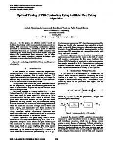
Fig. 3. (a) Step response and disturbance rejection of type-III closed loop control system. (b) Frequency response of type-III closed loop control system.
the lower frequency range, [I], [2]. Setting kh = 1 and the 2k kh TvTr. tenn of w6 equal to zero leads to 7;= p . In similar fashion, setting the tenn of w4 equal to zero along with the aid of 7;, drives to 4Tf-4(Tn +Tv )TE +TnTv= O. By choosing
::'
Tv= nTE then Tn becomes Tn= 4�-=-1) TE. Note that n > 4 must Fig.
2.
hold by so that a feasible PI 2D control law is extracted. By substituting the definitions of the gains 7;, Tn, Tv into the closed loop transfer function results in
Open loop frequency response of type-III closed loop control system.
respectively. For controlling troller
(I)
the proposed PID type con
(I+sTn)(1 +sTv) (1 +s1'x) C(s)= 2 s 7;(1+STEel)(1+STEe2) is employed [I], [2]. Note that the product khC(S) G(S)
(2)
T(s)=
4n(n-1)Tb2 +(n2 -4) TEs+n-4 . [ Sn(n-1)Tt,s4 +Sn(n-I) TtS3 +4n(n-I) TfS2J +(n2 -4) TES +(n-4)
Nonnalizing the time by setting
T(s')
(openloop transfer function) contains three free integrators so that the final closed-loop control system is of type-III. For determining controller parameters according to the Symmetrical Optimum criterion, zero-pole cancellation has to be achieved. In that, by setting 1'x= Tpl and assuming that TEe= TEe +TEe2, I TECJ TEe2 � 0, the transfer function of the control loop is equal to
s'= STE,
(
(6) becomes
4n(n-I) S,2 +(n2 -4) s'+(n-4) - [Sn(n-l)s'4 +sn(n-I)s'3 +4n(n-I)s' 2+]' (n2-4)s'+(n-4)
_
(7) The control loop defined in (7) is of type-III. This is justified by the equality of the tenns of P, j = 0, 1, 2, ao= bo, al= bl, a2= b2 of the closed-loop transfer function. In Fig. 3, the respective step Fig. 3(a) and frequency responses Fig. 3(b) of (7) are presented for two different values of parameter n. In s2kpTnTv +skp (Tn +Tv)+kp addition, in Fig.2 the open loop frequency response is shown, T(s)= [7;TmTEs4 +7;Tms3 +s2kpkhTnTv+skpkh(Tn+Tv) 1' from which we conclude that the magnitude of the closedloop transfer function IT(ju)1 is practically independent of the +kpkh ) parameter n. Moreover, sensitivity IS(ju)1 becomes maximum where TE = TEe +TEp. Since the magnitude of (3) is given by if n= 4.1 and minimum, if n= 7.46. In that case, (n= 7.46) r-----------:---------- Tn = Tv holds by. For every other value of parameter n, the shape of the open loop frequency response is preserved exactly k �(1-TnTv(2)2 +k �(Tn +Tv)2W 2
IT(jW) I=
[(kpkh(Tn +Tv) ]2' [7;TmTEW4+ ]2 +w2 kpkh(l-TnTvw2) -7;Tm(2) (4) and the denominator of (4) is defined by D(w)= (7;TmTE)2 w8 +7;Tm (7;Tm - 2kpkhT"TvTE) w6 +kpkh [27;TmTE - 2(Tn +Tv) 7;Tm +kpkhT2n T2v ] W4, +(kpkh)2 (T2n +T2v ) w2 +(kpkh)2 Fig. (5)
one way to optimize the magnitude of (4) is to set the terms of wj, j= 2,4, 6, . . ., in (5), equal to zero, starting again from
d,b)
d(s)
,(s)
y,(5)
4. Two degrees of freedom controller. Controller Cex(s) filters the reference input so that the undesired overshoot at the output y( s) is diminished. Controller Cex(s) affects the closed loop transfer function T(s) and not the output disturbance transfer function So(s)
882
=
£th.
3
1.8 1.6 1.4
0V� � 4iiJ,%' ..... ./...: .
where Po =1. The analysis proceeds by considering a general purpose time constant CI. Normalizing the time by setting s' = SCI polynomials in (11), all terms of s become x = '*, Y =
............: ....... f'IP:C.·.c::f· .. ···c.... : :·f·; .................
: .................. : ................. :
i·················
+
.................. :
......... '1 .........
:
1
........ !1
Fig. 8. Amplitude of the pulse with alternate sign is 5% of the value of the operating point. A series of pulses with alternate sign is imposed at the reference input. During the first step, an external filter is used Cex( s) to avoid the big overshoot at the output of the control loop.
Note that x depends only on the process parameters. If the process transfer function is completely known, then by solving (27), x, ti, y are easily calculated through (26). Since in many industry applications there is little a-priori knowledge regarding the qj coefficients, the PID controller is given the form
Cx (S')
1 +xs'+ !.x2st 2 l+s'x+st 2y - sI3t( (1 +s'tpn) - !kpkh� s'3(1 +S'tpn ) 8 x-q] _
)
(
(28)
according to the analytical expressions. Since the optimal overshoot that the closed loop control system has to exhibit, is not also known a-priori, the PID controller (28) will be tuned such, so that the overshoot of the closed loop control system is the mean value of the overshoot distribution shown in section IV. This value is equal to ovsref 77%. For doing the tuning, the control scheme of Fig.7 is adopted. The steps of the tuning are as follows. Step 1: Determination of the gain kp. The gain kp is determined from the step response of the plant at steady state. =
lim y(t)
Hoo
=
. hmsG(s)u(s)
s-tO
=
. hm s
s-tO
kp
-
1
n (1 +sTp ) s n
j=1
}
(29)
Fig. 10. Step response of the closed loop control system (black) optim �l tuning of the PID controller based on a known process model, (gray) automabc tuning of the PID controller, transfer function is not known. Input Disturbance di(S) is applied at 'r = 40 and output disturbance do(s) is applied at 'r = 80.
measured. Assuming that tPn Too an estimation of ql is given by ql r l +d PI +d � Therefore, (28) is initialized as follows =
=
=
Cx (s')
=
=
(
.
1 +xs 1 + '21 .x2s 1 2 tss )' I SI3(I+SI 100 � kPk h x4
) x-it
(30)
Initial value for x is selected x > � so that tix >O. Step 2: Tuning of the controller. At step k, OVSact is measured and compared with ovsref 77%. The error is fed into the PI controller (gray box)1 which tunes the parameter x. If at step k, OVSact < ovsref then at step k+1, x(k+1) >x(k). Note also that y is automatically tuned through y(k+ 1) !x2(k+1) and therefore y (k+1) >y (k). Also, if at step k+1, x (k+1) > x(k) then according to Fig.9, tl(k+ 1) < tl(k). Therefore, if x(k+l) >x(k) then ovsact(k+l) >ovsact(k) at the next pulse since zeros of the controller Cx are increasing and the integrator's time constant decreases. Tuning of Cx is terminated when overshoot of y(s) reaches the ovsref 77%. =
=
=
Step 2: Controller initialization. Feedback path is set to kh ] Its parameters are selected so that fast tuning of the controller's parameters 1 and also settling time tss of the step response of the process is Cx is achieved. =
885
6
VII.
A method for automatic tuning of the PID controller param eters has been presented for type-III control loops. The method assumes no a-priori knowledge of the plant transfer function as it frequently happens in many industry applications. It is based on the development of an optimal control law for PID type-III control loops. Its application to a large class of known process models shows that the shape of the step response in terms of the overshoot of the output is preserved. Since the optimal control law leads to a coupled relation via analytical expressions regarding P, I and D parameters, the controller gains can be expressed finally as a function of only one parameter. To this end, automatic tuning of the PID controller becomes finally an issue of tuning only one parameter.
12.5 .
10 . . ..........................
7.5
.
.
optimal tuning. PID. .
5 .
.
\t
:
· �· ..
0
,#
#�
"
r('r)�T.. . , ..
2.5
0
.
. .•#.
2.5
5
7.5
12.5
10
15
T
=
CONCLUSION AND OUTLOOK
tlTr
Fig. I I. Ramp response of the closed loop control system. (black) optimal tuning (gray) automatic tuning (gray-dotted) reference.
VIII.
ACKNOWLEDGMENT
This research was performed at the Department of Electrical & Computer Engineering, Aristotle University of Thessaloniki, Greece and is not a statement by ABB Switzerland Ltd.
120
Y(T)
ApPENDIX
100 .
Let the closed-loop transfer function be defined by (31),
80
T(s)
60
=
I 2 bms"'+bm Is"'- + .. ·+b 2 S +bl s+bo 2 n 1 ans"+an_IS - + ...+a2s +a ls+a o
(31)
�.
where m � nand T(s) By applying the Symmetrical Optimum criterion to (31) we will force IT(s) I � 1 in the wider possible frequency range. Thus, by setting s jro into (31) and =
40
:�i�:;:� =
squaring IT(jro) I leads to IT(jro)12 or finally if we make equal the terms of roj,(j 1 , 2 , . . . , n) in polynomials ID(jro)iZ, IN(jro)iZ so that IT(s)1 � 1 in the wider possible
20
0
=
=
0
2
4
8
6
10
T
=
tlTr
frequency range results in
ao
=
bo
(32)
a - 2a2ao
=
b - 2b2bO
a - 2a3al +2a4ao
=
T b� - 2b3bl +2b4b O b �+2blb5- 2b6bo
(33)
Fig. 12. Parabolic response of the closed loop control systems. (black) optimal tuning (gray) automatic tuning (gray-dotted) reference.
VI.
NUMERICAL RESULTS
For testing the proposed method, we compare the step response of the control loop for which the optimal control law has been applied after complete a-priori knowledge of the transfer function with the step response of the automatically tuned controller. 2 For filtering the reference, external controller of the form Cex (s') ';S'x has been considered. All time 1 constants have been normalized with s' STE where TE TEp+ TEe. In the example below, the plant transfer function =
=
is described by
G(s)
=
(1+0.65s)(1+0.8s) 5 e- s. (l+s)5
=
From Fig.lO it
is apparent that the step response based on optimal tuning is better than the response based on automatic tuning in terms of robustness, disturbance rejection and reference tracking. Settling time of output disturbance rejection is tss 21. 72 't'. Since the control loop is of type-III in both cases, perfect tracking of both ramp and parabolic signals is achieved, Fig. 1I. =
2Tuning based on overshoot 77%.
886
(
T
�
�
a +2ala5- 2a6ao -2a4a2
) ( =
-2b4b2
)
(34) (35)
REFERENCES [ I] Papadopoulos K.G., Papastefanaki E., Margaris N., "Optimal Tun ing of PID Controllers for Type-III Control Loops", Proceedings of 19'h Mediterranean Conference on Control and Automation, pp.l2951300, MED' I I, 20 I I. [2] Papadopoulos K.G., Margaris N.I, "Extending the Symmetrical Opti mum Criterion to the design of PID type-p control loops", Journal of Process Control, Elsevier, vo1.22, No I, pp. I I-25, 2012. [3] KJ. Astrom, T. Hagglund, C.C Hang, w.K. Ho, "Automatic tuning and adaptation for PID controllers - a survey", Control Engineering Practice, voU, No.4, pp.699-714, 1993. [4] R. Muszynski, Deskur 1., "Damping of Torsional Vibrations in High Dynamic Industrial Drives", IEEE Trans. on Ind. Electron., vol. 57, No. 2, pp. 544-552, 2010. [5] C. Kessler, "Das Symmetrische Optimum", Regelungstechnik, pp. 395400 und 432-426, 1958. [6] Oldenbourg R. c., Sartorius H., "A Uniform approach to the optimum adjustment of control loops", Trans. of the ASME, pp.1265-1279, 1954.