Autonomic Management of Reconfigurable Embedded Systems ...

Autonomic Management of Reconfigurable Embedded Systems using Discrete Control: Application to FPGA Xin An, Eric Rutten, Jean-Philippe Diguet, Nicolas Le Griguer, Abdoulaye Gamatié

To cite this version: Xin An, Eric Rutten, Jean-Philippe Diguet, Nicolas Le Griguer, Abdoulaye Gamatié. Autonomic Management of Reconfigurable Embedded Systems using Discrete Control: Application to FPGA. [Research Report] RR-8308, INRIA. 2013.

HAL Id: hal-00824225 https://hal.inria.fr/hal-00824225v3 Submitted on 11 Oct 2013

HAL is a multi-disciplinary open access archive for the deposit and dissemination of scientific research documents, whether they are published or not. The documents may come from teaching and research institutions in France or abroad, or from public or private research centers.

L’archive ouverte pluridisciplinaire HAL, est destinée au dépôt et à la diffusion de documents scientifiques de niveau recherche, publiés ou non, émanant des établissements d’enseignement et de recherche fran¸cais ou étrangers, des laboratoires publics ou privés.

RESEARCH REPORT N° 8308 May 2013 Project-Teams Ctrl-A, Lab-STICC and LIRMM

ISSN 0249-6399

Xin An, Eric Rutten, Jean-Philippe Diguet, Nicolas le Griguer, Abdoulaye Gamatié

ISRN INRIA/RR--8308--FR+ENG

Autonomic Management of Reconfigurable Embedded Systems using Discrete Control : Application to FPGA

Autonomic Management of Reconfigurable Embedded Systems using Discrete Control : Application to FPGA Xin An, Eric Rutten, Jean-Philippe Diguet, Nicolas le Griguer, Abdoulaye Gamatié Project-Teams Ctrl-A, Lab-STICC and LIRMM Research Report n° 8308 — May 2013 — 24 pages

Abstract: This paper targets the autonomic management of dynamically partially reconfigurable hardware architectures based on FPGAs. Such hardware-level autonomic computing has been less often studied than at software-level. We consider control techniques to model the considered behaviours of the computing system and derive a controller for the control objective enforcement. Discrete Control modelled with Labelled Transition Systems is employed in this paper. Such models are amenable to Discrete Controller Synthesis algorithms that can automatically generate a controller enforcing the correct behaviours of a controlled system. A general modelling framework is proposed for the control of FPGA based computing systems. We consider system application described as task graphs and FPGA as a set of reconfigurable areas that can be dynamically partially reconfigured to execute tasks. We encode the computation of an autonomic manager as a DCS problem w.r.t. multiple constraints and objectives e.g., mutual exclusion of resource uses, power cost minimization. We validate our models and manager computations by using the BZR language and an experimental demonstrator implemented on a Xilinx FPGA platform. Key-words: Control

Hardware Architectures, Dynamically Partially Reconfigurable FPGA, Discrete

RESEARCH CENTRE GRENOBLE – RHÔNE-ALPES

Inovallée 655 avenue de l’Europe Montbonnot 38334 Saint Ismier Cedex

Gestion Autonomique des Systèmes Embarqués Reconfigurables utilisant le Contrôle Discret : Application aux FPGA Résumé : Nous traitons de la gestion autonomique des architectures matérielles dynamiquement et partiellement reconfigurables à base de FPGAs. Cette forme d’informatique autonomique au niveau matériel a été peu étudiée comparé au niveau logiciel. Nous considérons des techniques de contrôle pour modéliser les comportements du système de calcul et pour dériver un contrôleur pour le maintien de l’objectif de contrôle. Nous utilisons des techniques de contrôle discret modélisé avec des systèmes de transitions étiquetées. Ces modèles se prêtent à une algorithmique de synthèse de contrôleurs discrets (SCD) qui peut générer automatiquement un contrôleur qui force les comportements corrects d’un système contrôlé. Un cadre général de modélisation est proposé pour le contrôle des systèmes informatiques à base de FPGA. Nous considérons que l’application est décrite par un graphe de tâches, et le FPGA comme un ensemble de zones reconfigurables, qui peuvent être dynamiquement et partiellement reconfigurées pour exécuter des tâches. Nous formulons le calcul d’un gestionnaire autonomique comme un problème de SCD concernant des contraintes et objectifs multiples, par exemple, l’exclusion mutuelle de l’utilisation des ressources, la minimisation du coût en énergie. Nous validons nos modèles et les calculs du gestionnaire en utilisant le langage BZR et un démonstrateur expérimental mis en œuvre sur une plate-forme FPGA Xilinx. Mots-clés : Architectures matérielles, FPGA reconfigurable dynamiquement et partiellement, contrôle discret

3

Autonomic Management of FPGA Embedded Systems using Discrete Control

Contents 1 Control of autonomic hardware

3

2 Background notions 2.1 FPGA-based architectures . . . . . . . . . . . . . . . . . . . . . . . . . . . . . . . 2.2 Discrete control . . . . . . . . . . . . . . . . . . . . . . . . . . . . . . . . . . . . . 2.3 Discrete control as MAPE-K . . . . . . . . . . . . . . . . . . . . . . . . . . . . .

4 4 5 6

3 DCS for managing DPR architectures 3.1 DPR FPGAs . . . . . . . . . . . . . . . . . . . . . . . . . . . . . . . . . . . . . . 3.2 System modelling as a DCS problem . . . . . . . . . . . . . . . . . . . . . . . . . 3.3 BZR encoding and DCS . . . . . . . . . . . . . . . . . . . . . . . . . . . . . . . .

8 8 10 16

4 Experimental results 4.1 Experimental validation . . . . 4.1.1 Case study . . . . . . . 4.1.2 Controller integration . 4.1.3 System implementation 4.2 Scalability . . . . . . . . . . . .

17 17 17 18 18 19

. . . . .

. . . . .

. . . . .

. . . . .

. . . . .

. . . . .

. . . . .

. . . . .

. . . . .

. . . . .

. . . . .

. . . . .

. . . . .

. . . . .

. . . . .

. . . . .

. . . . .

. . . . .

. . . . .

. . . . .

. . . . .

. . . . .

. . . . .

. . . . .

. . . . .

. . . . .

. . . . .

. . . . .

5 Related work

22

6 Conclusion and Perspectives

22

1

Control of autonomic hardware

Controlling FPGAs. We apply the autonomic framework to the context of FPGAs (Field Programmable Gate Arrays), hardware devices that compute a logic function by configuring its gates in a programmable way. A recent progress is dynamically partially reconfigurable (DPR) FPGAs. They support partial reconfigurations where only part of gates are reconfigured and reconfigurations to be performed at runtime. Autonomic computing has been seldom applied to such hardware systems, though they represent a significant case of its relevance. Control for autonomic management. We adopt control techniques to design the MAPEK (Monitor, Analyse, Plan, Execute, based on Knowledge). Formal models are used to describe the possible behaviours of the system under design, and control objectives giving the adaptation policy are specified separately. A controller is then derived based on the system models and objectives. The use of classical control techniques and models, typically these based on continuous time dynamics and differential equations, has been explored for various computing systems [8] and sometimes applied for hardware architectures [6]. A similar approach can be adopted by using discrete control techniques, where systems are considered from the viewpoint of events and states. The behaviours can then be modelled in the form of Petri nets or automata for, typically, synchronisation or coordination [17]. Discrete control for autonomic FPGAs. In this paper, we apply discrete control for the autonomic management of DPR FPGA based embedded systems. A systematic modelling framework is proposed, where system application behaviour, task implementations and executions, architecture reconfigurations and environment are modelled separately by using Labelled Transition Systems (LTS) or automata. Discrete Controller Synthesis (DCS) supported by a programming language and synthesis tool has been applied to compute an autonomic manager. RR n° 8308

4

An & Rutten & Diguet & Le Griguer & Gamatié

A video processing system has been implemented on a Xilinx FPGA platform to validate our proposal. Some results in the research report have been published in [2]. Section 2 recalls the backgrounds on FPGA architectures, discrete control and its relation to MAPE-K. Section 3 presents our modelling and autonomic manager computing framework through an illustrative example. Section 4.1 describes a real-life case study. Section 5 discusses related work, and Section 6 concludes.

2 2.1

Background notions FPGA-based architectures

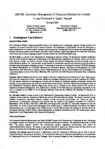
Basic reconfigurable cell. A FPGA is composed of an array of logic cells and programmable routing channels to implement custom hardware functionalities. The basic components of a logic cell are the LUT: a memory used as a programmable device to implement any logic function between inputs and outputs of a cell, and the D flip-flop: to hold a state between two clock cycles. A program consists of one or more bitstreams, which are binary files storing information to configure the LUTs and the routing switches. The bitstreams are generated by design tools such as the Xilinx Embedded Development Kit (EDK), which includes a tool suite called Xilinx Platform Studio (XPS) used to design an embedded system. Recent large FPGAs contain more than 200K logic cells that can be combined and interconnected to implement very complex designs. Multi-core architectures with tens of large hardware accelerators and processors can be implemented. Run-time partial reconfiguration. In the new generation of FPGAs, the hardware configuration can be updated at run-time by using the partial reconfiguration feature. A portion or region of the FPGA which implements some logic functions can be swapped with another one. If multiple functions are called sequentially, the same region can be reused so that the required size can be minimised. The best advantage of this type of reconfiguration is its ability to reconfigure hardware during the running of the static part, i.e., the part which does not contain any reconfigurable area. It assumes that the hardware reconfiguration does not disturb the execution of the application. The bitstreams therefore cover only some regions of the FPGA array. Such DPR FPGAs make them suitable for addressing constraints on resources (re-using some areas for different functions for applications that can be partitioned into phases) by adapting resources to available parallelism according to environment variations. DPR FPGAs represent a trade-off in that they are slower than dedicated Application-Specific Integrated Circuit (ASIC) hardware, but much faster than software running on general purpose CPUs. Management of reconfiguration. From a technical viewpoint, each hardware configuration file used for the different implementations of the partially reconfigurable regions is stored into a compact flash card. It can be loaded with a processor (e.g. microblaze, which is a 32-bit soft-core processor as implementable on Xilinx FPGAs). It performs the reconfiguration using the ICAP (Internal Configuration Access Port) as in Figure 1. The runtime management of reconfiguration involves a control loop, taking decision according to events monitored on the architecture, choosing the appropriate next configuration to install, and executing appropriate reconfiguration actions. The architecture dynamism increases the design complexity, for which a complete tool-chain is lacking [14]. Due to the relative novelty of DPR technologies, the management of reconfiguration has to be designed manually for important parts. Amongst different approaches to address this issue, we investigate the adoption of an autonomic computing approach for the design of reconfiguration control. The MAPE-K structure is Inria


5

FPGA CHIP STATIC REGION

Other HW

Softcore Microblaze

RECONFIGURABLE REGION

ICAP

Compact Flash Card Figure 1: FPGA with a microblaze softcore. based on behavioural models (in the form of automata) for the knowledge about the reconfigurability of these hardware platforms, and discrete control techniques for designing the adaptation policies.

2.2

Discrete control

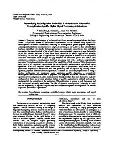
Automata and data-flow nodes. We first briefly introduce the basics of the automata-based modelling framework using formalisms from [1]. Behaviours are modelled in terms of Finite State Machines (FSM), or more precisely Labelled Transition Systems (LTS). They are defined by a finite set of states, between which there are transitions (from source state to target state) with a label of the form c / a: a firing condition c and an action a. When the FSM is in some current state, if there is a transition for which the condition is true, then it is taken and the next current state will be the target state. At the same time the action part will take the value true. Figure 2(a) illustrates this in the case of the control behaviour of a delayable task. It describes the control of a delayable task, which can either be idle, waiting or active. When it is in the initial Idle state, the occurrence of the true value on input r requests the starting of the task. Another input c can either allow the activation, or temporarily block the request and make the automaton go to a waiting state. Input e notifies termination. The outputs represent, resp., a: activity of the task, and s: triggering starting operation in the system’s API. As a concrete specification tool, we use the Heptagon programming language [4]. It supports the programming of mixed synchronous data-flow equations and automatawith parallel and hierarchical composition. The basic behaviour is that at each reaction step, values in the input flows are used, as well as local and memory values, in order to compute the values in the output flows for that step. Inside the nodes, this is expressed as a set of equations defining, for each output and local, the value of the flow, in terms of an expression on other flows, possibly using local flows and state values from past steps. Figure 2(a) shows a small program in this language, encoding exactly the FSM of Figure 2(a). Such automata and data-flow reactive nodes can be reused by instantiation, and composed in parallel (noted formally "|", and in the concrete syntax ";") and in a hierarchical way, as illustrated in the body of the node in Figure 2(c), with two instances of the delayable node. They run in parallel: one global step corresponds to one local step for every node. The compilation produces executable code in target languages such as C or Java, in the form of an initialisaRR n° 8308

6


node delayable(r,c,e:bool) returns (a,s:bool) let automaton state Idle do a = false ; s = r and c until r and c then Active twotasks(r1 , e1 , r2 , e2 ) | r and not c then Wait = a1 , s1 , a2 , s2 state Wait do a = false ; s = c enforce not (a1 and a2 ) until c then Active with c1 , c2 state Active do a = true ; s=false

delayable(r,c,e) = a,s a = false

a = false r and not c

Idle

e

Wait

r and c/s c/s Active

a)

a = true

b)

until e then Idle end tel

(a1 , s1 ) = delayable(r1 , c1 , e1 ) ;

c)

(a2 , s2 ) = delayable(r2 , c2 , e2 )

Figure 2: Delayable task: a) graphical / b) textual syntax; c) exclusion contract. tion function reset, and a step function implementing the transition function of the resulting automaton. It takes incoming values of input flows gathered in the environment, computes the next state on internal variables, and returns values for the output flows. It is called at relevant instants from the infrastructure where the controller is used. Control and contracts. The formalism of LTSs can be used to apply discrete controller synthesis (DCS), a formal operation on automata [3, 12]: given a FSM representing possible behaviours of a system, its variables are partitioned into controllable ones and uncontrollable ones. For a given control objective (e.g., staying invariably inside a subset of states, considered "good"), the DCS algorithm automatically computes, by exploration of the state graph, the constraint on controllable variables, depending on current state, for any value of the uncontrollables, so that remaining behaviours satisfy the objective. This constraint is inhibiting the minimum possible behaviours, therefore it is called maximally permissive. Algorithms are related to model checking techniques for state space exploration. BZR (http://bzr.inria.fr) extends Heptagon with a new behavioural contract [4]: its compilation involves DCS. Concretely, the BZR language allows for the declaration, using the with statement, of controllable variables, the value of which are not defined by the programmer. These free variables can be used in the program to describe choices between several transitions. They are then defined, in the final executable program, by the controller computed by DCS, according to the expression given in the enforce statement. BZR compilation invokes a DCS tool, and inserts the synthesised controller in the generated executable code, which has the same structure as above: reset and step functions. Figure 2(c) shows an example of contract coordinating two instances of the delayable node of Figure 2(a). The twotasks node has a with part declaring controllable variables c1 and c2 , and the enforce part asserts the property to be enforced by DCS. Here, we want to ensure that the two tasks running in parallel will not be both active at the same time: not (A1 and A2). Thus, c1 and c2 will be used by the computed controller to block some requests, leading automata of tasks to the waiting state whenever the other task is active. The constraint produced by DCS can have several solutions: the BZR compiler generates deterministic executable code by giving priority, for each controllable variable, to value true over false, and between them, by following the order of declaration in the with statement.

2.3

Discrete control as MAPE-K

Figure 3(a) shows the MAPE-K architecture of an autonomic system with a loop defining basic notions of Managed Element (ME) and Autonomic Manager (AM). The managed element, system or resource is monitored through sensors. An analysis of this information is used, in combination with knowledge about the system, to plan and decide upon actions. These reconInria

7


control

analyse monitor sensor

a)

plan

knowledge

execute

inputs

actuator

sensor

b)

managed element

transition function outputs state

inputs

actuator

sensor

c)

managed element

transition function outputs state actuator

managed element

Figure 3: Autonomic system: a) the MAPE-K manager; b) FSM autonomic manager; c) controllable AM. figuration operations are executed, using as actuators the administration functions offered by the system API. Self-management issues include self-configuration, self-optimisation, self-healing (fault tolerance and repair), and self-protection. Autonomic managers work in closed loop: for this, one design methodology is to apply techniques from Control Theory [8], with the advantage of ensuring interesting properties on the resulting behaviour of the controlled system e.g., stability, convergence, reachability or avoidance of some evolutions. In most cases, continuous models are used, typically for quantitative aspects. More recently, some works relied on Discrete Event Systems (DES), using supervisory control [3], typically for logical or synchronisation purposes e.g., deadlock avoidance in multithreaded programs [17]. They are based on reactive systems models such as Petri nets or Finite State Machines (FSM), which we also call automata. As shown in Figure 3(b), this instantiates the general autonomic loop with knowledge on possible behaviours represented as a formal state machine, and planning and execution in the form of the automaton transition function with a control output, which will trigger the actuator. Basic features required for a system to be managed in an autonomic fashion have been identified in previous work e.g., in the context of component-based autonomic management [15]: for an ME to be manageable it must be observable and controllable. The manager transforms flows of observations into flows of control choices and actions. Observability translates into outputs, as shown by dashed arrows in Figure 3(c) for an FSM AM, exhibiting (some) of the knowledge and sensor information (raw, or analysed); this can feature state information on the AM itself or of MEs below. Controllability translates to having the AM accept some influence on the decision, and it corresponds to additional input for control, as in Figure 3 for an FSM AM. Its values can be used in the guards and exhibit choices between different transitions. This builds up to a hierarchical framework as in the structure shown in Figure 4. Given that AMs have been made observable and controllable, an upper-level AM can perform their control

inputs

transition function outputs state

control

inputs sensor

control


inputs sensor


managed element

Figure 4: Autonomic coordination for multiple AMs. RR n° 8308

8


coordination using their additional control input to enforce a policy. Considering the case of FSM managers makes it possible to encode the coordination problem as a DCS problem. The controller of this upper-level AM is synthesised by DCS.

3

DCS for managing DPR architectures

3.1

DPR FPGAs

We present informally the class of computing systems of interest through an illustrative example. They are inspired by the self-adaptive embedded systems in [6]. However, we address the problem in a different and original way. Hardware architecture. We consider a multiprocessor architecture implemented on an FPGA (e.g. Xilinx Zynq device), which is composed of a general purpose processor A0 (e.g. ARM Cortex A9), and a reconfigurable area divided into four tiles: A1–A4 (see Figure 5). The communications between architecture components are achieved by a Network-on-Chip (NoC). Each processor and reconfigurable tile implements a NoC Interface (NI). A fixed dual port memory buffer is associated with each tile, which means that at most two tasks can simultaneously access data stored in the shared memory. Reconfigurable tiles can be combined and configured to implement and execute tasks by loading predefined bitstreams, such as tiles A1 and A2 of Figure 5. The architecture is equipped with a battery supplying the platform with energy. Regarding power management, an unused reconfigurable tile Ai can be put into sleep mode with a clock gated mechanism such that it consumes a minimum static power. NI NI Mem. Buffer

NI A1

A2

Mem. Buffer

A0 Mem. Buffer

A4

A3

Mem. Buffer

NI

NI NoC

Figure 5: Architecture structure and execution example.

Application software. We consider system functionality described as a directed, acyclic task graph (DAG). A DAG consists of a set of nodes representing the set of tasks to be executed, and a set of directed edges representing the precedence constraints between tasks. Note that we do not restrict the abstraction level of tasks associated with the nodes, and a task can be an atomic operation, or a coarse fragment of system functionality. Figure 6 shows an example consisting of four tasks. In our framework, we suppose each task performs its computation with the following four control points: • being requested or invoked; • being delayed: requested but not yet executed; • being executed: to be executed on the architecture; Inria


9

B A

D C

Figure 6: DAG application specification.

• notifying execution finish, once it reaches its end. Occurrences of control points being requested and notifying finishes depend on runtime situations, and are thus unpredictable and uncontrollable. The way of delaying and executing tasks is taken charge by a runtime manager aiming to achieve system objectives. Task implementation. Given a hardware architecture, a task can be implemented in various ways characterised by various parameters of interest, such as used reconfigurable tiles (ur), worst case execution time (WCET) (wt), and power peak pp. For example, two implementations of task A can be: • A on A1: wt = 50, pp = 20; • A on A3 + A4: wt = 10, pp = 30; In this preliminary work, we assume that WCET represents the time cost induced from the start of bitstream loading to the end of task execution. Among the possible task implementations, a runtime manager is in charge of choosing the best implementation at runtime according to system objectives.

task B

task B

or task C

task A 1)

2)

task C 3)

Figure 7: Configurations and reconfigurations.

System reconfiguration. Figure 7 shows three system configuration examples. In configuration 1, task A is running on tiles A3 and A4 while tiles A and B are set to the sleep mode. Configurations 2 and 3 show two scenarios with tasks B and C running in parallel. Once task A finishes its execution according to the graph of Figure 6, the system can go to either configuration 2 or configuration 3 depending on the system requirements. For example, if the current state of the battery level is low, the system would choose configuration 2 as configuration 3 requires the complete FPGA working surface and therefore consumes more power. RR n° 8308

10


System objectives. System objectives define the system functional and non-functional requirements. This section gives the objectives considered in the paper, and categorises them as logical and optimal control objectives. Generally speaking, logical objectives concern state exclusions, whereas optimal objectives target the states associated with optimal costs. Considered logical control objectives are as follows: 1. resource usage constraint: exclusive uses of reconfigurable areas A1-A4; 2. dual accesses to the shared memory (i.e., at most two functions running in parallel); 3. energy reduction constraint: switch areas to (a) sleep mode when executing no task; (b) active mode when needed; 4. reachability: system execution can always finish once started; 5. power peak constraint: power peak of hardware platform is constrained w.r.t battery levels; Optimal control objectives of interest are as follows: 6. minimise power peak of hardware platform; 7. minimise WCET of system executions; 8. minimise worst case energy consumption of system executions.

3.2

System modelling as a DCS problem

We specify the modelling of the computing system behaviour and control in terms of labelled automata. System objectives are defined based on the models. We focus on the management of computations on the reconfigurable tiles and dedicate the processor area A0 exclusively to the resulting controller. Architecture behaviour. The architecture (see Figure 5) consists of a processor A0, four reconfigurable tiles {A1, A2, A3, A4} and a battery. Each tile has two execution modes, and the mode switches are controllable. Figure 8(a) gives the model of the behaviour of tile Ai. The mode switch action between Sleep (Sle) and Active (Act) depends on the value of the Boolean controllable variable c_ai . The output acti represents its current mode. RMi c_ai

acti = false c_ai Slei not c_ai

a)

Acti acti = true

BM down

down

acti

up

b)

H st=h

down M

up

st=m

L up

st

st=l

Figure 8: Models RMi for tile Ai, and BM for battery.

Inria

11


The battery behaviour is captured by the automaton in Figure 8(b). It has three states labelled as follows: H (high), M (medium) and L (low). The model takes input from the battery sensor, which emits level up and down events, and keeps track of the current battery level through output st. Application behaviour. Software application is described as a DAG, which specifies the tasks to be executed and their execution sequences and parallelism. We capture its behaviour by defining a scheduler automaton representing all possible execution scenarios. It does so by keeping tracking of application execution states and emitting the start requests of tasks in reaction to the task finish notifications. Sdl eB

req eA,eB,eC,eD

I

req/rA

A

eA/rB,rC

C

eC/rD

eB and eC/rD

B,C eC

B

D

eD

T

rA,rB,rC,rD

eB/rD

Figure 9: Scheduler automaton Sdl capturing application execution behaviours. Figure 9 shows the scheduler automaton of the application in Figure 6. It starts the execution of the application by emitting event rA , which requests the start of task A, upon the receipt of application request event req in the idle state I. Upon the receipt of event eA notifying the end of A’s execution, events rB and rC are emitted together to request the execution of tasks B and C in parallel. Task D is not requested until the execution of both B and C is finished, denoted by events eB and eC . It reaches the final state T , implying the end of the application execution, upon the receipt of event eD . Scheduler Automaton Derivation. The scheduler automaton or LTS of a DAG described application captures the dynamic execution behavior of the application. Its states represent the tasks that are executing. They are denoted and labeled by the names of these tasks. It has an initial state I, i.e., the idle state, which means the application has not been invoked, and an end state T , which means that the application has finished its execution. The automaton input events are the task end events ei and the application request event req, while its output events are the task request events ri . Its transitions are of the form g/a, where g is a firing condition, and a is an action. A firing condition is a boolean expression of input events, and an action is a conjunction of output events. Note: 1) we suppose the application is only invoked once. If it is allowed to be repeatedly invoked, the end state would be the same to the initial state. 2) if the graph has a task that has more than one instance, the instances are then seen as different tasks by the algorithm. Algorithm 1 illustrates how to construct the scheduler automaton for a DAG. It derives the automaton from initial state I to end state T by exploring the state space of the application execution w.r.t. the DAG. • Inputs: a directed, acyclic task graph < T, C >, where T and C represent respectively the set of tasks, the set of edges. • Local variables and functions used in the algorithm: s: a state, with element label represents the tasks executing, and element taskSet to represent the set of tasks associated to RR n° 8308

12


the state (i.e., executing in the state); stateQueue: a FIFO queue, keeping track of the states to be processed, with functions popup(), add(s) to return and delete the first state element, and add state s to the end of the queue; readyT askSet: ti .prec: the set of tasks immediately precedes ti ; traversed(s): a function returns the states from I to s (included), which represents the tasks that have finished and executing, with taskSet to return union of tasks associated with each state; drawTrans(source,sink,trans. label), drawState(I); drawnStates: the states that have been drawn out; toState(task set): to associate/label the task set with the state; tc: a set of tasks, or a task combination; powerSet(tc): the power set of tc - ∅. At line 1, the initial state, i.e., idle state I is drawn denoted by drawn(I). The set of drawn states drawnStates is thus initialized to {I} at line 2. State queue stateQueue stores the states that have been drawn but not processed. It is initialized to have element I at line 3. Variable readyT askSet represents the set of tasks that are enabled to execute once some event happens. A task is enabled if all its precedent tasks have finished their executions. Lines 4 to 8 set readyT askSet to the set of tasks that have no precedent tasks, as such tasks can be executed immediately once the application is invoked/requested denoted by the receipt of event req. Lines 9 to 41 deal with the sequential processing of the states stored in stateQueue. The processing of a state concerns the drawing of its immediate following states and the transitions, and put the new drawn states in the queue. The automaton derivation finishes when the queue becomes empty. In the following, we describe how state s from queue stateQueue is processed. Line 10 evaluates the first state of the queue to s and removes it from the queue. Three types of states are distinguished and processed accordingly. They are initial state I, end state T and the rest. Lines 12 to 16 deal with the processing of idle state I. The algorithm firstly computes its following state nextState by evaluating the readyT askSet (got from Lines 4 to 8) to its taskSet at line 12. nextState represents the state once the application is invoked. Line 13 draws the state, and line 14 draws the transition from state I to nextState with label req/{ri |ti ∈ readyT askSet}, where ri is the request event of task ti , denoted by drawT rans(I, nextState, req/rreadyT askSet ). Lines 15 and 16 add nextState to drawnStates and the end of stateQueue. If state s is the end state (line 17), the algorithm simply proceeds. Lines 20 to 39 deal with the processing of state s that represents the application executing state between I and T . In general, the algorithm explores all the possible subsets of the executing tasks in s (denoted by s.taskSet), and computes the following states accordingly. powerSet(s.taskSet) represents the power set of s.taskSet without ∅. Given an element tc which represent a subset of the executing tasks in s, lines 21 to 38 deal with the drawing of the following states of s w.r.t. the simultaneous finishes of the executions of tasks in tc. Lines 21 to 26 compute the tasks that would become enabled if the set of tasks tc finishes. Variable readyT askSet initialized to ∅ at line 21 is used to keep these tasks. Function traversed(s) represents the set of states (in the drawn automaton so far) that are traversed by some path from state I to state s (I and sincluded). The union of the task sets associated with traversed(s) denoted by traversed(s).taskSet thus represents the tasks that have been executed before reaching s and are executing in current state s. At line 22, the algorithm explores the tasks that have not been requested (denoted by T −traversed(s).taskSet) to find out readyT askSet once tc finishes. Lines 23 to 25 decides whether ti is enabled once tc finishes and adds ti to readyT askSet if it is. ti is enabled if the set of its precedent tasks is a subset of the union of tasks that have finished (denoted by traversed(s) − s.taskSet) and the tasks would finish denoted by tc. At line 27, nextState denotes the state following s due to the tasks in tc simultaneously finish. Its taskSet thus equals to the union of computed readyT askSet and the tasks that are still executing in s after tc finishes denoted by s.taskSet − tc. If nextState.taskSet is ∅, this means that once Inria


13

Algorithm 1 Scheduler Automaton Derivation 1: drawState(I); 2: drawnStates = {I}; 3: stateQueue = stateQueue.add(I); 4: for all ti ∈ T do 5: if ti .prec = ∅ then S 6: readyTaskSet = readyTaskSet ti ; 7: end if 8: end for 9: while stateQueue! = ∅ do 10: s = stateQueue.popup(); 11: if s = I then 12: nextState.taskSet = readyTaskSet; 13: drawState(nextState); 14: drawTrans(I, nextState, req/r SreadyT askSet ); 15: drawnStates = drawnStates nextState; 16: stateQueue.add(nextState); 17: else if s = T then 18: continue; 19: else 20: for all tc ∈ powerSet(s.taskSet) do 21: readyTaskSet = ∅; 22: for all ti ∈ T − traversed(s).taskSet do S 23: if ti .prec ⊆ (traversed(s).taskSet S - s.taskSet) tc then 24: readyTaskSet = readyTaskSet ti ; 25: end if 26: end for S 27: nextState.taskSet = readyTaskSet (s.taskSet - tc); 28: if nextState.taskSet = ∅ then 29: nextState = T; 30: end if 31: if nextState ∈ drawnStates then 32: drawTrans(s, nextState, etc ); 33: else 34: drawState(nextState); 35: drawTrans(s, nextState, etc );S 36: drawnStates = drawnStates nextState; 37: stateQueue.add(nextState); 38: end if 39: end for 40: end if 41: end while

the tasks in tc finish, no more task can become enabled or is still executing, i.e., all tasks have finished executions and nextState is the end state T (lines 28 to 30). In a scheduler automaton, a state might have more than one precedent states. The algorithm thus checks, at line 31, if nextState has been drawn. If it has, only the transition needs to be drawn from s to nextState with label {eti |ti ∈ tc denoted by etc at line 32. Otherwise, the algorithm draws both state RR n° 8308

14


nextState and the transition at lines 34 and 35, and then updates drawnStates and stateQueue accordingly. Task execution behaviour. In consideration of the four control points of task executions (see Section 3.1), the execution behaviour of task A associated with two implementations (see Section 3.1) can be modelled as Figure 10. It features an initial idle state IA , a wait state WA , and two 1 2 executing states XA , XA corresponding to two implementations of task A. Controllable variables are integrated in the model to encode the controllable points: being delayed and executed. Upon the receipt of start request rA , task A goes to either: i i • executing state XA , i ∈ {1, 2} if the value of controllable variable ci leading to XA is true, or W • wait state WA if delayed, i.e., the value of Boolean expression c = ci , i ∈ {1, 2} is false.

TMA es=I

rA,eA

eA rA, c1

({A1}, c1,c2 50,20)

XA1 es=XA1

({},⊥,0)

IA

rA, not c

c1 es=W

WA

eA rA, c2 c2

({},⊥,0)

({A3,A4}, es 10,30) XA2 es=XA2

Figure 10: Execution behaviour model T MA of task A. i From wait state WA , upon the receipt of event ci , it goes to execution state XA . When the execution of task A finishes, i.e., the end notification event eA is received, the automaton goes back to idle state IA . Output es represents its execution state. Local execution costs. The execution costs of different task implementations are different. Three cost parameters are considered (see Section 3.1). We capture them by associating cost values denoted by a tuple (rs, wt, pp) with the states of task models, where: rs ∈ 2RA (RA is the set of architecture resources), wt ∈ N (a WCET value) and pp ∈ N (a power peak). The costs associated with executing states are the values associated with their corresponding implementations. For idle and wait states, apparently rs = ∅, pp = 0. However, the wt values for idle and wait states depend on the execution times of their precedent tasks. We therefore represent it by using a special symbol ⊥, and thus we have wt ∈ N∪ ⊥. Figure 10 gives the complete local model of task A.

Global system behaviour model. The parallel composition of control models for reconfigurable tiles RM1 -RM4 , battery BM and tasks T MA -T MD , plus scheduler Sdl comprises the system model: S = RM1 |...|RM4 |BM |T MA |...|T MD |Sdl with initial state q0 = (Sle1 , ..., Sle4 , H, IA , ..., ID , I). It represents all the possible system execution behaviours in the absence of control (i.e., a runtime manager is yet integrated). Each execution behaviour corresponds to a complete path, which starts from initial state q0 and reaches one of the final states: Qf = (q(RM1 ), ..., q(RM4 ), q(BM ), IA , ..., ID , T ), Inria


15

where q(Id) denotes an arbitrary state of automaton Id. Global costs. The costs defined locally in each task execution model need to be combined into global costs. Costs on states. A system state q is a composition of local states (denoted by q1 , ..., qn ), and we define its cost from the local ones as follows: • used resources: union of used resources associated with the local states, i.e., rs(q) = S rs(qi ), 1 ≤ i ≤ n; • worst case execution time: this indicates how much time the system takes at most in this current state. It is thus defined as the minimal WCET of all executing tasks in this state, i.e., wt(q) = min(wt(qi ), wt(qi ) 6=⊥, 1 ≤ i ≤ n); Otherwise, if no task is executing in the state, i.e., ∀1 ≤ i ≤ n, wt(qi ) =⊥, wt(q) = 0; P • power peak: the sum of values associated with the local states, i.e., pp(q) = (pp(qi ), 1 ≤ i ≤ n); • worst case energy consumption: the product of the worst case execution time and power peak of the system state, i.e., we(q) = pp(q) ∗ wt(q). Costs on paths. We also need to define the costs associated with paths so as to capture the characteristics of system execution behaviours. Given path p = qi → qi+1 → ... → qi+k , and costs associated with system states, we define corresponding costs on path p as follows: P • WCET: the sum of WCETs on the states along the path, i.e., wt(p) = wt(qj ), i ≤ j ≤ i + k; • power peak: the maximum value on the states along the path, i.e., pp(p) = max(pp(qj ), i ≤ j ≤ i + k); • worst case energy consumption: the Psum of the worst case energy consumptions on the states along the path, i.e., we(p) = we(qj ), i ≤ j ≤ i + k. System objectives. The two types of system objectives: logical and optimal ones, can then be described in terms of the states and the costs defined on the states or paths of the model. Logical control objectives. For any system state q, we want to enforce the following: T (1) exclusive uses of reconfigurable tiles by tasks: ∀qi , qj ∈ q, i 6= j, that rs(qi ) rs(qj ) = ∅; (2) dual accesses to shared memory, i.e., at most two functions can access the memory at the same time: P 1 qi ∈ Xi vi ≤ 2, s.t. vi = , where Xi represents the set of executing states of 0 otherwise corresponding task; (3.a) switch tile Ai to sleep mode, when executing no task: @qi ∈ q, Ai ∈ rs(qi ) ⇒ acti = f alse; (3.b) switch tile Ai to active mode when executing task(s): ∃qi ∈ q, Ai ∈ rs(qi ) ⇒ acti = true; (4) reachability: Qf is always reachable. (5) battery-level constrained power peak (given threshold values P0 , P1 , P2 ): pp(q) < P0 (resp. P1 and P2 ) when battery level is high (resp. medium and low). RR n° 8308

16


Optimal control objectives. Such objectives can be further classified into two types of objectives: one-step optimal and optimal control on path objectives. We use pseudo functions max and min in the following to represent the maximisation and minimisation objectives, respectively. One-step optimal objectives. One-step optimal objectives aim to minimise or maximise costs associated with states and/or transitions in a single step [12]. Objective 4 of Section 3.1 belongs to this type. (6) minimise power peak pp in next states of state q: min(pp, q). Optimal control on path objectives. Such objectives aim to drive the system from the current state to the target states Qf at the best cost [5]. Objective 5 and 6 are such objectives. (7) minimise remaining WCET wt from state q: min(wt, q, Qf ); (8) minimise remaining energy consumption we from q: min(we, q, Qf ).

3.3

BZR encoding and DCS

Given the system graphical models and objectives of Section 3.2, this section describes the controller synthesis by using BZR and the DCS tool Sigali. Logical and optimal objectives are treated differently. BZR encoding of the system model. The automaton encoding of system components in Section 3.2 can be translated to textual encoding easily as Figure 2. The BZR encoding of the global system behaviour can then be obtained by composing all these models. Finally, the costs on system states are defined as described in Section 3.2 (not detailed here, due to space limitation). Enforcing logical control objectives. BZR contracts are able to directly encode the logical control objectives of Section 3.2. The following shows the BZR contract. 1 2

contract var exclusive_tileA1, idle_tileA1, swt_sleep_tileA1, swt_act_tileA1, bound_pp: bool; 3 let (*exclusive usage of tile A1*) 4 exclusive_tileA1 = idle_tileA1 or only_A_on_tileA1 or ... or only_D_on_tileA1; 5 idle_tileA1 = not A_on_tileA1 & not B_on_tileA1 & not C_on_tileA1 & not D_on_tileA1; 6 only_A_on_tileA1 = A_on_tileA1 & not B_on_tileA1 & not C_on_tileA1 & not D_on_tileA1; (*switch to sleep mode when running no task*) 7 swt_sleep_tileA1 = not idle_tileA1 or not act1; (*switch to active mode when executing a task*) 8 swt_act_tileA1 = idle_tileA1 or act1; (*bounded power peak*) 9 bound_pp = if battery_high then (pp