In this tutorial we will discuss how two separate neural network approaches can solve a simple AVO problem. In doing so, we will shed light on several important ...
AVO classification using neural networks
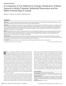
AVO classification using neural networks: A comparison of two methods Brian H. Russell, Laurence R. Lines, and Christopher P. Ross1 ABSTRACT In a previous paper (Russell et. al., 2002), the authors applied the multi-layer perceptron (MLP) neural network to the solution of a straightforward AVO classification problem. In this paper, we will summarize the earlier work, and then show how the problem can be solved in an alternate fashion by using the radial basis function neural network (RBFN). By using an AVO model as our input, we are able to gain greater insight into the inner workings of neural networks. INTRODUCTION In this tutorial we will discuss how two separate neural network approaches can solve a simple AVO problem. In doing so, we will shed light on several important questions: why are some neural networks only able to solve linear problems, whereas others can solve nonlinear problems, and how can neural networks be trained to do these tasks? The two types of neural networks that we will use are the multi-layer perceptron (MLP), which is sometimes called the multi-layer feed forward network (MLFN) (Hampson et al, 2001), and the radial basis function neural network (RBFN). The AVO problem that we will train the networks to solve is the recognition of a class 3 anomaly on an AVO attribute crossplot. As we shall see, training a computer to perform tasks that are simple for a human being (that is, an interpreter) can often be quite difficult. However, if we can train a computer to systematically and objectively interpret an AVO crossplot it will be worth the effort. THE AVO PROBLEM The basic AVO interpretation problem that we will study is differentiating between the AVO responses of the two reservoirs shown in Figure 1. Figure 1(a) shows a wet sand encased between two shale layers, and Figure 1(b) shows a gas sand encased between the same two shales. The P-wave velocity (VP), S-wave velocity (VS), and density (ρ) for each layer are shown in each figure. We will assume that the far angle of incidence is small enough (i.e. approximately 30°) that we can ignore the third term in the Aki-Richards equation and write the reflectivity as a function of angle of incidence θ as R(θ ) = A + B sin 2 θ , (1) where A is the AVO intercept, and B is the AVO gradient. Appendix A gives the full expressions for A and B as a function of V P , VS , ρ and angle.
CREWES Research Report — Volume 14 (2002)
1
Russell, Lines, and Ross
(a)
(b)
FIG. 1: Two simple geological models where (a) shows a wet sand between two shale layers and (b) shows a gas sand between the same two shales.
Using the values for VP, VS, and density ρ shown in Figure 1, we can now work out the values for the AVO intercept and gradient for the wet and gas sands. Let's start with the wet sand, noting that the VP/VS ratio in both the sand and shale layer is equal to 2. As shown in Appendix A, this leads to the simplification that B = − A for both the top and base of the layer using the parameters shown in Figure 1 gives ATOP_WET = BBASE_WET = +0.1 and ABASE_WET = BTOP_WET = -0.1. For the gas sand, the VP/VS ratio is equal to 1.65, and the intercept does not simplify as it did the wet sand. However, the calculation is still straightforward, and leads to ATOP_GAS = BTOP_GAS = -0.1 and ABASE_GAS = BBASE_GAS = +0.1. Note that, for the gas case, A=B for both the top and base of the layer. The AVO curves for the wet and gas cases are shown in Figure 2, for an angular aperture of 0º to 30º. It is observed that the absolute values of the gas sand curves show an increase in amplitude, whereas the absolute values of the wet sand curves show a decrease in amplitude. Model AVO Curves 0.15 Amplitude
0.10 0.05 0.00 -0.05 -0.10 -0.15 0
5
10
15
20
25
30
Angle (degrees) Top Gas
Base Gas
Top Wet
Base Wet
FIG. 2. This figure shows the AVO responses from the top and base interfaces of the wet and gas sands shown in Figure 1.
2
CREWES Research Report — Volume 14 (2002)
AVO classification using neural networks
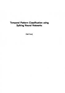
For this neural network tutorial, the parameters have been selected to minimize the mathematics. However, these values do fall within a reasonable petrophysical range encountered where class 3 geologies occur. After scaling each of the values of A and B by a factor of 10 (to give values of +1 and -1) they have been put on an A-B crossplot, as shown in Figure 3(a). In our example, the wet points (shown as solid blue circles) establish the wet sand-shale trend, and the top and base gas (shown as solid red circles) plot in the other two quadrants of the A-B crossplot. This is a typical class 3 AVO anomaly (Rutherford and Williams, 1989), caused by gas saturation reducing the sand impedance and the Vp/Vs ratio of the sand encased in the shale.
(a)
(b)
FIG. 3. Intercept versus gradient crossplots, where (a) shows the crossplot of the A and B values from the wet and gas models of Figure 1, crossplotted after being scaled by a factor of 10, and (b) shows a Gulf of Mexico real data example, where the grey ellipse shows the “wet trend” and the gold and blue ellipses show the top and base of the pay sand, respectively.
Despite the simplicity of the model, the plot shows us what is expected in a noise-free AVO crossplot. For comparison, Figure 3(b) is an interpreted AVO A-B crossplot for a class 3 AVO response in the Gulf of Mexico (Ross, 2000). The centre grey ellipse encompasses all of the wet sand-shale AVO points while the gold and blue ellipses outlying the grey “wet trend” points are associated with the top and base of the pay sand, respectively. Identifying the wet trend and the outlying two points in Figure 3(a) is a trivial problem for the eye to interpret. However, as we will see in the next section, the early neural networks could not properly address situations as simple as this, and technology improvements (often through trial and error) were required to eventually solve the problem. Let us now have a quick overview of the various types of neural networks.
CREWES Research Report — Volume 14 (2002)
3
Russell, Lines, and Ross
INTRODUCTION TO NEURAL NETWORKS Before going into the specific details of neural networks, and how they can be used to solve the AVO problem defined earlier, it is important to step back and describe some of their general properties. First of all, what is a neural network? The simplest answer is that a neural network is a mathematical algorithm that can be trained to solve a problem that would normally require human intervention. Although there are many different types of neural networks, there are two ways in which they are categorized: by the type of problem that they can solve and by their type of learning. The two main types of problems that a neural network can solve are the classification problem and the prediction problem. In the classification problem, the input dataset is divided into a series of classes, such as sand, shale and carbonate, or gas, wet and oil, etc. In the prediction problem, a parameter of interest is predicted from a number of input values. For example, we could use a series of input seismic attributes to predict reservoir porosity at each seismic sample (Hampson et al., 2001). It should be clear that the problem that we wish to solve here is a classification problem, in which we want to classify sands as either wet or gas-charged, based on their input AVO attributes. Once we have decided on the type of problem to solve, we need to teach the neural network how to solve the problem, which is called network learning. The two main ways in which a neural network can learn are called supervised and unsupervised learning. In supervised learning, we present the neural network with a set of inputs and outputs for a particular problem, and let it determine the relationship between these inputs and outputs. The advantage of supervised learning is that we can interpret the output, since we have specified its nature. The disadvantage is that we need a sufficient number of input and output values to be able to adequately train the network. Examples of neural networks that use the supervised learning technique are the MLP and RBFN referred to earlier. In unsupervised learning, we present the neural network with a series of inputs and let the neural network look for patterns itself. That is, the specific outputs are not required. The advantage of this approach is that we do not need to know the answer in advance. This disadvantage is that it is often difficult to interpret the output. An example of this type of unsupervised technique is the Kohonen Self Organizing Map (KSOM) (Kohonen, 2001). Next, we will discuss the basics of the perceptron, which is the basic building block of the multi-layer perceptron neural network, and discover its limitations for solving our AVO problem. THE PERCEPTRON The classic model of the neuron is called the perceptron (McCulloch and Pitts, 1943) and is illustrated in Figure 4. The perceptron accepts N inputs a1 , a 2 ,… , a N , and produces a single output. Mathematically, the perceptron has two separate stages. First, the inputs are weighted and summed according to the equation:
x = w1 a1 + w2 a 2 + … + w N a N + b
4
CREWES Research Report — Volume 14 (2002)
(2)
AVO classification using neural networks
The last weight, b, is called the bias, and is often written as w0. Next, a threshold function f is applied to the intermediate output x to product the final output y, or y = f (x ) (3)
FIG. 4. The figure above shows the perceptron neural network for N inputs and a single output. The two boxes enclosed by the dashed line constitute the perceptron.
The choice of the threshold function f is important and depends on the problem being solved. If f(x) = x, the perceptron reduces to a linear sum of the inputs. In many applications, f(x) is set to the smoothly varying sigmoidal function such as the hyperbolic tangent function, which is defined as: e x − e−x f (x ) = x (4) e + e−x A graph of the hyperbolic tangent function is shown in Figure 5(a). Hyperbolic Tangent Function 1
f(x)
0.5
0
-0.5
-1 -3
-2
-1
0
1
2
3
x
(a)
(b)
FIG. 5. This figure shows a graph of (a) the hyperbolic tangent function of Equation (4), and (b) the symmetric step function of Equation (5).
For a two class problem, such as the one we are discussing here, we often use the step function, which is given mathematically by the equation:
CREWES Research Report — Volume 14 (2002)
5
Russell, Lines, and Ross
+ 1, x ≥ 0 f (x ) = − 1, x < 0
(5)
A graph of the symmetric step function is shown in Figure 5(b). Now, let's consider how to adapt the perceptron to our AVO problem, as shown by the neural network graph in Figure 6. We have reduced the problem to two inputs, the intercept (A) and gradient (B), and are using is the symmetric step function to compute the final output. The step function is a logical and convenient choice because A and B have scaled values of ±1. However, the interpretation of the output values will be different than the input. A value of +1 will indicate the presence of a gas sand and a value of –1 will indicate the presence of a wet sand.
FIG. 6: The perceptron adapted to the AVO problem of Figure 3, where the inputs are the intercept (A) and gradient (B) and the function shown schematically is the symmetrical step function.
Notice that the equation for intermediate output x is now given as x = w1 A + w2 B + b
(6)
The key question is: how do we determine the weights w1, w2, and b? To answer this, let us take an intuitive look at what these weights mean. From equation (6), it is obvious we are interested in the separation between x < 0 and x > 0 , which occurs when x = 0 . This is called the decision boundary, and is illustrated in Figure 7 for the general case. To find out where this boundary crosses the A and B axes, we simply need to successively set A and B to zero, to give
B=
−b −b , and A = . w2 w1
Figure 7 shows the weight vector w = (w1, w2)T, which is always normal to the decision boundary and points in the direction of f(x) = +1. We chose f(x) = +1 because in this quadrant we want to separate the wet sand response from the base of the gas sand. This will therefore give us the signs of w1 and w2.
6
CREWES Research Report — Volume 14 (2002)
AVO classification using neural networks
FIG. 7: The perceptron decision boundary. Note that either b or w1 and w2 must be negative to make the resulting intercept value on the A and B axes positive.
It is important to note from Figure 7 that the perceptron can only separate points that are linearly separable. That is, for a two dimensional case we can draw a line between the points, and for a three-dimensional case we can draw a plane. (For higher dimensional inputs we use hyperplanes to separate the points, which are simply the mathematical extension of the plane to higher dimensions.) This limitation meant that the perceptron could not solve a simple Boolean algebra problem, the exclusive OR, or XOR (Haykin, 1998). It turns out that this problem is identical to the AVO problem that was discussed earlier. We will therefore address our AVO problem rather than the XOR problem. So, let's now revisit the AVO problem of Figure 2, as shown in Figure 8. First of all, notice that we will not be able to separate both the top and base of the gas sand from the wet trend with a single decision plane, since this is a nonlinear separation problem. Thus, we must choose to separate either the top of the gas sand, as shown in Figure 8(a), or the base of the gas sand, as shown in Figure 8(b). To solve for the weights for the top of the gas sand, notice that
A=B=−
(a)
b b =− = −1 . w1 w2
(b)
FIG. 8: The AVO problem from Figure 2 with decision boundaries, where (a) shows separation of the base of the gas sand and (b) shows separation of the top of the gas sand.
CREWES Research Report — Volume 14 (2002)
7
Russell, Lines, and Ross
Although b, w1 and w2 can be scaled by any value, it is best to choose the simplest values, which are w1 = w2 = −1 , and therefore b = −1 . The perceptron diagram for this is shown in Figure 9(a).
(a)
(b)
FIG. 9: Perceptron implementations of separating (a) the top of gas (Perceptron 1), and (b) the base of gas (Perceptron 2).
Next, to solve for the weights for the base of gas sand, notice that: b b =− = +1 w1 w2 Therefore, the weights are w1 = w2 = +1 and b = −1 . This is shown in Figure 9(b). Table 1 shows that these values do indeed solve the problem for the four possible cases. A=B=−
Table 1: The table above shows the outputs from the perceptron models of Figure 9.
Inputs
Sand
A
B
Perceptron 1
Perceptron 2
x1
y1
x2
y2
-1
-1
+1
+1
-3
-1
Base Wet
-1
+1
-1
-1
-1
-1
Top Wet
+1
-1
-1
-1
-1
-1
Base Gas
+1
+1
-3
-1
+1
+1
Top Gas
Although we have solved for the top and bottom of the gas sand individually we have still not solved the complete problem, which is to separate the gas sand responses from the wet sand responses. This requires a multi-layer perceptron, or MLP. THE MULTI-LAYER PERCEPTRON
8
CREWES Research Report — Volume 14 (2002)
AVO classification using neural networks
The problem that we encountered in the last section, that perceptrons can only solve linearly separable problems, was also encountered by the early neural network researchers. This dealt a severe blow to the enthusiasm for neural networks. Although the solution now appears quite straightforward (since hindsight is 20/20) it took almost forty years from the initial development of the perceptron for this new technique to be widely introduced (McClelland and Rumelhart, 1981). The solution is to add a second layer of perceptrons. In Figure 10 we have shown a two-layer perceptron with N inputs into M neurons. The sum and function boxes of our earlier figures have been replaced by a single box, but that the perceptrons still has the same internal workings as previously described. Notice that the first set of weights now have two subscripts and a superscript, written as w(k)ij, where i represents the perceptron number, j represents the input number and the superscript k in brackets indicates the layer number. This figure is pervasive in many neural network papers, but how do we interpret it? More importantly, why can a second layer solve a nonlinear problem, whereas a single layer of perceptrons only solve a linear problem?
FIG. 10: A multi-layer perceptron with N inputs, M perceptrons, and a single output.
To answer these questions, we need to recast the AVO problem of Figure 3 as a multi-layer perceptron, similar to Figure 11. In this neural network, the inputs are still the intercept (A) and gradient (B), but now they are both interconnected, via the weights, to the two perceptrons.
CREWES Research Report — Volume 14 (2002)
9
Russell, Lines, and Ross FIG. 11: The multi-layer perceptron for the gas-water sand model of Figure 3.
Mathematically, the two-layer perceptron can be written as the following matrix equation. y ( 2 ) = f ( 2 ) ( W ( 2 ) f ( 1 ) ( W ( 1 )a + b( 1 ) ) + b( 2 ) ) ,
(7)
where ( j) w11 y1 a1 ( j) y a w 2 2 ( j) y= = 21 ,a = ,W " " " ( j) wM ( j ) 1 yN a N
( j) w12 ( j) w22 "
wM( j( )j ) 2
b1( j ) ( j) , b ( j ) = b2 , " ( j) ( j) # wM ( j ) N bM ( j ) # # $
w1( Nj ) w2( Nj ) "
and the superscript refers to the layer number. To go beyond the mathematics, we will now present an intuitive development of what happens in a multi-layer network. What we have done is simply connect two perceptrons to produce two separate outputs. These outputs now represent the input to a new perceptron. If we use the two perceptrons from Figure 9 as our two first layer perceptrons, we can crossplot their outputs y1(1) and y2(1), and design a new perceptron, p(2), to separate these outputs. This is shown in Figure 12, using the output values from Table 1. The base gas and top gas points have moved to what was the wet trend on the input points, but both of the wet sands have moved to the point (-1, -1), which was the top gas point for the input. This new linearly separable problem is graphically shown by the decision boundary on Figure 13. Thus, we can derive the weights for perceptron p(2) in Figure 12, which are: b ( 2) b ( 2) − ( 2 ) = − ( 2 ) = −1 , w1 w2 or w1( 2 ) = w2( 2) = b ( 2) = +1 .
10
CREWES Research Report — Volume 14 (2002)
AVO classification using neural networks FIG. 12: A crossplot of the outputs of the two perceptrons of Figure 9.
The final perceptron, with weights, is shown in Figure 13. Notice that the weights are all equal to +1 or –1, which are the simplest set of weights but that there are many other sets of weights that would solve the problem.
FIG. 13: The final multi-layer perceptron weights.
To verify that this indeed is the solution, Table 2 then shows the outputs for all possible inputs. As we can see in Table 2, the correct output is given for all four input cases. Thus, we have solved the problem of how to separate a simple Class 3 gas sand from its equivalent wet sand.
CREWES Research Report — Volume 14 (2002)
11
Russell, Lines, and Ross Table 2: The computed output values from the multi-layer perceptron in Figure 13 for the four input models of Figure 3, where y(2) shows that the gas sand values (+1) have been separated from the wet sand values (-1).
Inputs
Perceptron p1(1)
Perceptron p 2(1)
Perceptron p ( 2)
Sand
A
B
y1(1)
y 2(1)
y ( 2)
Top Gas
-1
-1
+1
-1
+1
Base Wet
-1
+1
-1
-1
-1
Top Wet
+1
-1
-1
-1
-1
Base Gas
+1
+1
-1
+1
+1
THE RADIAL BASIS FUNCTION APPROACH
In the previous section we applied the multi-layer perceptron (MLP) to the problem of classifying a Class 3 AVO anomaly. We discovered is that, although the problem is not linearly separable in its original form, it becomes linearly separable after transforming the input points with suitably chosen weights and activation functions, and thus can be solved using a MLP with a single hidden layer. In this section we will use a different type of neural network, the radial basis function network (RBFN) (Haykin, 1998), to solve the same problem. The RBFN is different than the MLP in that it uses “distance” in multi-dimensional space as a method of linear separation, rather than simply applying weights to the input points. By “distance” we mean the vector distance from the input points to some target value. We then apply a nonlinear function to this distance to achieve separation. To understand the differences between the MLP and the RBFN, recall that the basic equation behind the MLP is the linear equation wTx = 0
(8)
where wT = (w1, w2, …, wN) and xT = (x1, x2, …, xN). (Note that we have replaced the earlier notation in which a was the input vector with x, since we will no longer be using the concept of an intermediate output, for which x was used earlier.) That is, we look for a weight vector, w, which, when applied to the input vector, x, gives us the correct decision boundary, or hyperplane, as written in equation (8). Note that the bias can be included in w if we also append a value of 1 to the input vector x and rename the bias as w0 (earlier, b was used to annotate the bias). In the MLP approach, the linearly weighted sum in equation (8) was then passed through a nonlinear activation function, and then a second application of both equation (8) and the activation function
12
CREWES Research Report — Volume 14 (2002)
AVO classification using neural networks
was applied to the output of the first process. A different approach was suggested by Cover (1965), which in words can be written: “A complex pattern classification problem cast in a high-dimensional space nonlinearly is more likely to be linearly separable than in a low-dimensional space.” Mathematically, this can be written wTφ(x) = 0,
(9)
where φ = (φ1, φ2, ..., φΝ) is now some nonlinear function and equation (9) defines a hyperplane, or decision boundary, in φ-space. For example, if we take the simplest situation of separation between two classes, C1 and C2, then w T φ( x ) ≥ 0 ⇒ x ∈ C 1 ,
and
w T φ( x ) < 0 ⇒ x ∈ C 2 .
There are two crucial questions to be answered if we want to implement equation (9). First, what is the best choice for the function φ and, second, is the vector x simply equal to the input values? The answer to the first question, which can be derived either from statistical or regularization theory, is that the multivariate Gaussian is an optimal (but not the only) choice for the function φ. The answer to the second question is that we need to compare the input vectors to a set of pre-chosen centres, using the vector norm, or distance, as our fitting criterion. Thus, we can define a series of values φj such that x −c 2 i j , j = 1, 2 , … , M , i = 1, 2. … , N , φ j ( x i ) = exp − 2 σ where cj are the M centres, xi are the N input vectors, and σ is a scaling function.
(10)
As an example, let us return to the class 3 AVO problem. Recall that the four input vectors (i.e. N = 4) are: − 1 x1 = , − 1
+ 1 x2 = , − 1
+ 1 x3 = , − 1
+ 1 x 4 = . + 1
where points x1 and x4 are the top and base of the gas zone, respectively, and points x2 and x3 are the top and base of the wet zone, respectively. Let us define two centers (i.e. M = 2) using the gas sand values, or: − 1 + 1 c1 = , c 2 = . − 1 + 1
Let us also define
CREWES Research Report — Volume 14 (2002)
13
Russell, Lines, and Ross
x −c i j φij = φ j ( x i ) = exp − 2 σ
2
(11)
Note that in terms of the vector components we can rewrite the above equation as: (xi 1 − c j 1 )2 + (xi 2 − c j 2 )2 φij = exp − σ2
(12)
We will also let σ = 1. From the definitions of our input vectors and centers, we can see that there are only three possible distances d = x i − c j
2
. If the vector and center are
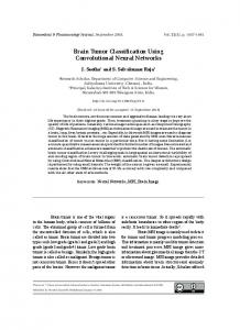
identical, we have d = 0. If one element of the vector is equal to one element of the center and the other is opposite, we have d = 4. Finally, if the vector and center are opposite in sign, we have d = 8. Therefore, the values of φij are: φ11 = φ42 = exp[− 0 ] = 1.0 , φ12 = φ41 = exp[− 8 ] = 0.0003 , and φ21 = φ22 = φ31 = φ32 = exp[− 4 ] = 0.018 . Grouping the terms, we get: φ11 1.0 φ12 0.0003 φ 0.018 and φ2 = φ 22 = 0.018 . φ1 = 21 = φ31 0.018 φ32 0.018 φ 41 0.0003 φ 42 1.0 Figure 14(a) shows the original AVO problem in A-B space, and Figure 14(b) shows a crossplot of φ 1 ( x i ) versus φ 2 ( x i ) . Notice that we have now achieved a linear separation between the gas sand values and the wet sand values. We will now extend this concept to develop the radial basis function neural network, and solve for the linear separation seen in Figure 14(b).
14
CREWES Research Report — Volume 14 (2002)
AVO classification using neural networks
(a)
(b)
FIG. 14: The AVO classification problem of Figure 3, where (a) shows the original problem in intercept-gradient space with the nonlinear decision boundary annotated, and (b) shows the same problem after transformation the φ1-φ2 space of equation (10).
Figure 15 next shows how the concepts of the previous section can be applied in neural network form. Note that this is a similar diagram to the MLP except for two important differences. First, there are no weights between the inputs and the application of the φ function in the first layer neurons. Second, although there are weights (and bias value) leading to the second layer neuron, there is no application of a nonlinear function at this neuron. In other words, the second layer is simply a linear sum.
FIG. 15: The radial basis function neural network (RBFN) implementation of the AVO classification problem, using the φ1-φ2 calculations of equation (10) and the implementation described below.
The RBFN is therefore much more straightforward to implement than the MLP and can be written mathematically as 2
y ( x i ) = w0 + ∑ w j φ j ( x i ),
i = 1, … , 4.
(13)
j =1
To solve for the weights, we set each output value to the training data values given in Table 1, where +1 indicated the presence of gas and -1 indicates the absence of gas.
CREWES Research Report — Volume 14 (2002)
15
Russell, Lines, and Ross
i 1 2 3 4
Ai -1 +1 -1 +1
Bi -1 -1 +1 +1
φi1
φi2
1 0.0003 0.018 0.018 0.018 0.018 0.0003 1
di +1 -1 -1 +1
Thus, we have four linear equations with three unknowns, as shown below: d1 d2 d3 d4
= w0 = w0 = w0 = w0
+ w1 φ11 + w2 φ12 + w1 φ21 + w2 φ22 + w1 φ31 + w2 φ32 + w1 φ41 + w2 φ42
This can be written as the following matrix equation:
d =Φ w,
(14)
where d 1 + 1 1 w0 1 d − 1 2 , w = w1 and Φ = d= = 1 d 3 − 1 w2 d 4 + 1 1
φ11 φ21 φ31 φ41
φ12 1 1 .0 0.0003 φ22 1 0.018 0.018 . = φ32 1 0.018 0.018 φ42 1 0.0003 1 .0
Since Φ is a non-square matrix with more rows than columns (i.e. more equations than unknowns), the problem is overdetermined, and the solution to equation (14) is given by the following equation:
(
w = Φ T Φ + λI
)
−1
ΦTd ,
(15)
where λ is a pre-whitening term and I is the identity matrix. For this problem, no prewhitening was needed, and the solution is as follows: − 1.076 w = 2.075 . 2.075
Recall from our discussion of the MLP that this means that the intercepts on both the A and B axes are given by the following ratio: –w0/w1 = – w0/w2 = - (- 1.076 / 2.075) = 0.519. These are the points where the dashed line in Figure 14(b) intersects each axis.
16
CREWES Research Report — Volume 14 (2002)
AVO classification using neural networks
We have therefore shown how to construct a linear separation boundary for our AVO classification problem using the radial basis function neural network, and found that the solution is actually more straightforward than the multi-layer perceptron approach. CONCLUSIONS
In this tutorial, we have shown how neural networks can be used to solve a simple Class 3 AVO classification problem. The simplicity of the model allowed us to derive the weights by hand for two types of neural networks, the multi-layer perceptron (MLP) and radial basis function neural network (RBFN). In doing so, we gained insight into both types of neural networks. First, a single layer perceptron can only solve a linearly separable problem. However, by adding a second layer of weights and perceptrons, as in the MLP, we can transform a nonlinear problem into a linear problem, and thus find the solution using an single output perceptron. On the other hand, the RBFN does not require a second layer of weights, and applies a nonlinear function to the initial input to perform the linear separation. In both cases, our simple AVO problem proved to be an ideal model for understanding the inner workings of the neural networks in question. In more complex problems, the weights for the MLP are derived using a technique called backpropagation, in which we try to reduce the error between the known output and the output created by a set of initial weights by backward propagation of the errors. This is fully described in Haykin (1998). REFERENCES Cover, T.M., 1965, Geometrics and statistical properties of systems of linear inequalities with application in pattern recognition, IEEE Transactions on Electronic Computers, EC-14, 326-334. Hampson, D. P., Schuelke, J. S. and Quirein, J. A., 2001, Use of multiattribute transforms to predict log properties from seismic data: Geophysics, Society of Exploration Geophysicists, 66, 220-236. Haykin, S.S., 1998, Neural Networks: A Comprehensive Foundation, 2nd Edition, Macmillan Publishing Company. Kohonen, T., 2001, Self Organizing Maps: Springer Series in Information Sciences, 20, Springer Verlag, Berlin. McClelland, J.L. and Rumelhart, D. E., 1981, An interactive model of context effects in letter perception: part 1: An account of the basic findings, Psychological Review 88: 375-407. McCulloch, W. S. and Pitts, W., 1943, A logical calculus of the ideas immanent in nervous activity: Bulletin of Mathematical Biophysics, 5, 115-133. Ross, C. P., 2000, Effective AVO crossplot modeling: A tutorial: Geophysics, Society of Exploration Geophysicists, 65, 700-711. Rutherford, S. R. and Williams, R. H., 1989, Amplitude-versus-offset variations in gas sands: Geophysics, Society of Exploration Geophysicists, 54, 680-688.
CREWES Research Report — Volume 14 (2002)
17
Russell, Lines, and Ross
APPENDIX A THE AKI-RICHARDS EQUATION
The Aki-Richards equation is given by: R(θ ) = A + B sin 2 θ + C sin 2 tan 2 θ ,
(A-1)
where A=
1 ∆VP ∆ρ is the intercept term, + 2 VP ρ
∆VS 1 ∆V P ∆ρ − 4γ − 2γ is the gradient term, VS ρ 2 VP 1 ∆VP is the curvature term, C= 2 VP B=
2
V γ = S , ∆VP = VP 2 − VP1 , ∆VS = VS 2 − VS 1 , ∆ρ = ρ2 − ρ1 , VP V + VS 2 V + VP 2 ρ + ρ1 VP = P1 , VS = S 1 , and ρ = 2 . 2 2 2
Assuming a small incident angle (< 30o) the third term can be dropped, and, if we assume that VP/VS = 2, or γ = 1/4, then the gradient can be simplified to B=
1 ∆VP ∆ρ ∆VS ∆ρ , − + + 2 VP ρ VS ρ
and we also find that
∆VP VP
=
∆VS VS
.
(A-2)
(A-3)
Substituting (A-3) into (A-2), we get:
B = −A
(A-4)
ACKNOWLEDGEMENTS
We wish to thank our colleagues at the CREWES Project and at Hampson-Russell Software for their support and ideas, as well as the sponsors of the CREWES Project.
18
CREWES Research Report — Volume 14 (2002)