Published in Proc. of the 12th European Signal Processing Conf. (EUSIPCO 2004), Sep. 6-10, 2004, Vienna, Austria
BAYESIAN SUBSPACE METHODS FOR ACOUSTIC SIGNATURE RECOGNITION OF VEHICLES Mario E. Munich Evolution Robotics Pasadena, CA 91103
[email protected]
ABSTRACT Vehicles may be recognized from the sound they make when moving, i.e., from their acoustic signature. Characteristic patterns may be extracted from the Fourier description of the signature and used for recognition. This paper compares conventional methods used for speaker recognition, namely, systems based on Mel-frequency cepstral coefficients (MFCC) and either Gaussian mixture models (GMM) or hidden Markov models (HMM), with Bayesian subspace method based on the short term Fourier transform (STFT) of the vehicles’ acoustic signature. A probabilistic subspace classifier achieves a 11.7% error for the ACIDS database, outperforming conventional MFCC-GMM- and MFCC-HMM-based systems by 50%. 1. INTRODUCTION All vehicles emit characteristic sounds when moving. These sounds may come from various sources including rotational parts, vibrations in the engine, friction between the tires and the pavement, wind effect, gears, fans. Similar vehicles working in comparable conditions would have a similar acoustic signature that could be used for recognition. The aim of acoustic signature recognition of vehicles is to apply techniques similar to automatic speech recognition to recognize the type of the moving vehicle, based on its acoustic signal. Automatic acoustic surveillance enables continuous, permanent verification of compliance with limitations of conventional armaments, as well as with peace agreements, tasks for which there could be insufficient personnel or where continuous human presence could not be easily accepted. Acoustic surveillance could also play a crucial role in the success of military operations. Several systems have been proposed for vehicle recognition [2, 4, 5, 10, 12] in the past. A common focus of these systems is placed on the analysis of fine spectral details from the acoustic signatures. However, it is difficult to compare these systems because both the databases and the experimental conditions (such as sampling rate, frame size, type of recognition recognition) are different. Choe et. al. [2] and Maciejewski et. al. [5] designed their systems based on wavelet analysis of the incoming waveforms and Neural Networks classifiers. Choe et. al. applied Haar and Daubechies-4 wavelets to feature signals selected by hand from audio data collected from 2 military vehicles. The audio data was sampled at 8 kHz and at 16kHz. A recognition rate of 98 % was obtained with statistical correlation for in-sample utterances. Maciejewski et. al. used Haar wavelets to preprocess audio data sampled at 5 kHz. Two different classifiers, a Radial Basis Function network with 8 mixture components and a multilayer perceptron, were utilized to identify a military vehicle out of 4 possible candidates. A recognition rate of 73.68% was achieved by the RBF in the classification of out-of-sample frames. Wu et. al. [12] applied short-time Fourier transform and principal components analysis (PCA) for vehicle recognition. The system worked with a sampling rate of 22 kHz. The feature vectors consisted of the normalized short-time Fourier transform of frames of the utterances. The recognition technique closely resembled the one proposed by Turk and Pentland [11] for face recognition; however, no experimental performance was shown in the paper.
Liu [4] described a vehicle recognition system that used a biological hearing model [13] to extract multi-resolution feature vectors. Three classifiers: learning vector quantization (LVQ), tree-structured vector quantization (TSVQ), and parallel TSVQ (PTSVQ), were evaluated on the ACIDS database. A recognition accuracy of 92.6 % was presented for classification of single frames in in-sample conditions. The accuracy increases to 96.4 % by using a block of four contiguous frames; however, the block recognition performance dropped to 69% when using out-of-sample testing data. Sampan [10] presented the design of a circular array of 143 microphones used to detect the presence and classify the type of vehicles. The acoustic signals were sampled at 44.1 kHz and separated in 20 msec. long windows. The array sensor was designed to work in high frequencies; therefore, audio frames were restricted to the frequency band [2.7 kHz, 5.4 kHz]. The feature vectors consisted of energy features extracted in this frequency band. Two different classifiers, a multi-layer perceptron and an adaptive fuzzy logic system, were used for vehicle recognition. Classification rates of 97.95 % for a two-class problem, 92.24 % for a four-class problem, and 78.67 % for a five-class problem were reported in this work. Incidentally, array microphones have also been successfully used for speaker recognition by Lin et. al. [3]. Recognition of acoustic signatures is usually performed in two steps. The first one, called front-end analysis, converts the captured acoustic waveform into a set of feature vectors. The second one, named back-end recognition, obtains a statistical model of the vehicle feature vectors from a few example utterances and performs recognition on any given new utterance. This paper compares the recognition performance of three different systems. Given the similarity between vehicle and speaker recognition, the first two systems represent the state-of-the-art in speaker recognition and provide a baseline performance. These two systems use a frontend based on Mel-frequency cepstral coefficients (MFCC). These feature vectors provide a spectral description of the signature by separating the spectral information into bands, followed by an orthogonalizing transformation, and a dimensionality reduction. The recognition back-ends are based on either Gaussian mixture models (GMM) [9] or hidden Markov models (HMM) [1]. These two systems use a coarse representation of the spectral information of the signature. In contrast with them, we propose a novel approach that pays close attention to fine spectral detail of the signatures. The feature vectors consist of the log-magnitude of the short term Fourier transform (STFT) of the acoustic signatures. These spectral vectors have sufficiently high dimensionality in order to provide a precise representation of the acoustic characteristics of the signature. However, estimation of probability density functions in high-dimensional spaces may be quite unreliable. The solution of the trade-off can be achieved by projecting the high dimensional feature vectors to a low dimensional subspace in which density estimation could be reliable performed. Recognition is then obtained with a probabilistic subspace classifier. The paper is organized as follows: section 2 describes the recognition systems, section 3 presents the experimental results, and section 4 draws some conclusions and describes further work.
2. RECOGNITION SYSTEMS 2.1 Feature extraction Mel-frequency cepstral coefficients (MFCC) have been originally proposed for speech recognition and speaker recognition (see e.g., Rabiner and Juang [8]). Incoming utterances are segmented into frames using a Hamming (or a similar type) window. The frame size is selected such that the signal within the window could be assumed to be a realization of a stationary random process and hence, the frequency content of the waveform can be estimated from the Fourier transform of the frame. Overlapping frames are used to correct for non-stationary audio portions captured within a given frame. The spectrum of each frame is computed with the fast Fourier transform (FFT). The resultant spectrum is then typically filtered by a filter bank whose individual filter’s center frequency is placed in accordance with the Mel frequency scale. The filter-bank output is used to represent the spectrum envelope. The next step is to apply the discrete cosine transform to the log of the filter-bank output. Finally, the feature vector is composed of few of the lowest cepstrum coefficients. The two baseline systems evaluated in this paper are based on an MFCC front-end. MFCC features may not be optimal for vehicle recognition since fine details of the spectral patterns are smeared out by the filter bank. Sometimes these details contribute to the success of recognition. The third recognition system works directly with the raw acoustic spectrum. Each utterance is segmented into frames using a Hamming window to reduce Gibbs effects in the spectrum. The feature vector is just the log-magnitude of the Fourier transform of each frame. Figure 1 shows the corresponding mean spectral frame for each vehicle in the ACIDS database, obtained using a window size of 250 msec. (256 points). 2.2 Probabilistic Modeling and Classification Both the GMM- and HMM-based baseline systems model the acoustic feature space in terms of mixtures of a number of Gaussian distributions. Typically the feature space is first divided into N classes. Each class has one centroid that can be obtained via vector quantization. Using the expectation-maximization (EM) algorithm, one can determine the means and variances of individual classes and thereby construct mixture models. An important difference between HMMs and GMMs is that an HMM usually has a left-to-right topology, while a GMM can be considered as an ergodic HMM where transitions are permitted from any state to any state (including itself). In other words, a GMM does not preserve time sequence information. The techniques used to compute the classification likelihoods are well-known (refer to [9, 1] for more information) and will not be described here. In the case of the third system, probability densities for either GMMs or HMMs models may not be reliable estimated since the feature vectors live in a high dimensional space. Hence, we project the high dimensional feature vectors to a low dimensional subspace that provides a good representation of the data. Principal component analysis (PCA) is a dimensionality reduction technique that extracts the linear subspace that best represents the data. PCA has been successfully employed for face recognition [11] and was proposed for vehicle recognition by Wu et. al. [12]. Given a training set of N-dimensional spectral vectors {xt ,t = 1, · · · , K}, the basis of the best-representation linear subspace is provided by the eigenvectors that correspond to the largest eigenvalues of the coK xt be the mean and let variance matrix of the data. Let µ = K1 ∑t=1 1 K Σ = K ∑t=1 (xt − µ)(xt − µ)T be the covariance of the training set; then Σ = U S U T is the eigenvector decomposition of Σ with U being the matrix of eigenvectors and S being the corresponding diagonal matrix of eigenvalues. The basis of the subspace is given by the columns of UM , the sub-matrix of U containing only the eigenvectors corresponding to the M largest eigenvalues. The feature vectors T (xt − µ). xt are represented in the PCA subspace by zt = UM Bayesian subspace methods for face recognition have been proposed by Moghaddam and Pentland [7] and have been shown to
outperform PCA methods [6]. A similar Bayesian subspace technique is used for vehicle recognition in this paper; the most relevant formulae is presented in the following paragraphs, refer to references [7, 6] for a full description of the method. Assuming that the mean µ and the covariance matrix Σ have been estimated from the training set and assuming a Gaussian density, the likelihood of a spectral vector x is given by: 1
P(x) =
T
e− 2 [(x−µ) (2π)
N 2
Σ−1 (x−µ)]
p
(1)
|Σ|
This likelihood can be estimated as a product of two marginal ˆ and independent Gaussian densities P(x) = PS (x)PˆS¯ (x), the true marginal density in the PCA subspace PS (x) and the estimated marginal density in the orthogonal complement of the PCA sub2 space PˆS¯ (x). Let ε 2 (x) = kxk2 − ∑M i=1 zi be the residual PCA re1 N construction error and let ρ = N−M ∑i=M+1 λi be the average of the ˆ eigenvalues of Σ in the orthogonal complement subspace, then P(x) is given by: 2 z2i )( ) ( − 12 ∑M − ε (x) i=1 λi e 2ρ e ˆ = = PS (x)PˆS¯ (x) (2) P(x) N−M 1 M (2πρ) 2 (2π) 2 ∏M λ 2 i=1 i
In a multiple classes (C1 ,C2 , · · · ,Cn ) recognition scenario, subspace density estimation should be performed for each class separately. Classification is performed by maximizing the likelihoods ˆ P(x|C i ) obtained with equation 2. 3. EXPERIMENTS The acoustic signature data set used in the experiments is the Acoustic-seismic Classification Identification Data Set (ACIDS) collected by the Army research laboratory. The database is composed by more than 270 data runs (single target) from nine different types of ground vehicles (see table 1) in four different environmental conditions (normal, dessert, and two different arctic environments). The vehicles were traveling at constant speeds that varied from 5 km/h to 40 km/h depending upon the particular run, the vehicle, and the environmental condition. The closest point of approach to the sound-capture system varied from 25 m to 100 m. The acoustic data was collected with a 3-element equilateral triangular microphone array with an equilateral length of 15 inch. The microphone recordings were low-pass filtered at 400 Hz with a 6th -order filter to prevent spectral aliasing and high-pass filtered at 25 Hz with a 1st -order filter to mitigate wind noise. The data was digitized by a 16-bit A/D at the rate of 1025.641 Hz. The distance between microphones generated a time delay in waveform arrival to the microphones. But the delay was smaller than 1 millisecond for all the conditions and hence, the delay was negligible for all practical purposes at the given sampling rate of 1025.641 Hz.
Type 1 Type 2 Type 3 Type 4 Type 5 Type 6 Type 7 Type 8 Type 9
heavy track vehicle heavy track vehicle heavy wheel vehicle light track vehicle heavy wheel vehicle light wheel vehicle light wheel vehicle heavy track heavy track
# runs 58 31 9 22 29 36 7 33 15
# recordings 174 93 27 66 87 108 21 99 45
Table 1: Vehicle types. The ACIDS database is composed of acoustic signatures from nine vehicles. The data is not equally distributed across vehicles: vehicles type 3 and 7 have much fewer examples than other vehicle types. The nine vehicles could be re-grouped in five categories (type 1-2, type 3-5, type 4, type 6-7, and type 8-9) according to the labels provided by the Army.
Vehicle 1
Vehicle 2
8
4
12 log spectrum
12 log spectrum
log spectrum
12
8
4 50
150
250 freq. (Hz)
350
450
50
150
350
450
50
4
8
4 250 freq. (Hz)
350
450
50
150
250 freq. (Hz)
350
450
log spectrum
log spectrum 150
250 freq. (Hz)
150
350
450
250 freq. (Hz)
350
450
350
450
12
8
4 50
50
Vehicle 9
12
4
450
8
Vehicle 8
8
350
4
Vehicle 7
12
250 freq. (Hz)
12 log spectrum
8
150
150
Vehicle 6
12 log spectrum
log spectrum
250 freq. (Hz) Vehicle 5
12
50
8
4
Vehicle 4
log spectrum
Vehicle 3
8
4 50
150
250 freq. (Hz)
350
450
50
150
250 freq. (Hz)
Figure 1: Mean spectral features. The solid line of the plots shows the mean spectrum for the corresponding vehicles. The dotted lines display a band that is one standard deviation apart from the mean. The value of the standard deviation is quite stable across frequencies and across vehicles. Characteristic spectral peaks are kept as salient features instead of being blurred out by the filter bank.
The ACIDS database was evenly divided into a training and a test set in order to evaluate the performance of the system with out-of-sample utterances. The division was made so that examples from all environmental conditions were allocated in both the training and test sets. Also, given that the microphone array provided three simultaneously-recorded utterances per run, all three recordings were assigned to either one of the sets. The three systems described in this paper classifies complete utterances as being produced by one of the vehicles. The classification of complete incoming utterances is very similar in all the systems. It starts by separating the audio data into frames in order to compute spectral feature vectors; then, the likelihood of each feature vector is computed for each of the vehicle models using the methods described in section 2.2; and finally, the complete utterance is classified using the total accumulated likelihood. The ACIDS database could be tested in a few different ways. On one hand, we can classify test utterances into the nine original vehicle types or we can classify it into the five classes defined by unique labels of the vehicles. On the other hand, the microphone array provided three simultaneous recording of utterances. We can classify each recording independently (single channel) or we can make a joint use of the three recordings (multiple channel) by aggregating individual classification results with a voting procedure. Table 2 presents the error rates of the systems for four testing conditions: 9-class single channel, 9-class multiple channel, 5-class single channel, and 5-class multiple channel. The MFCC feature vectors were extracted using 500 msec.-long overlapping windows with a frame rate of 200 msec. First 5 MFCC coefficients were obtained with a Hamming window frame segmentation followed by filtering the frame spectrum with an 8-channel triangular filter bank,
centered according to Mel-frequency, and a discrete cosine transform of the log-filter bank energies. The feature vector consisted of the 5 static MFCC coefficient plus frame energy. The GMM used a 32-mixture models and the HMM used a 3-state, 16-mixtureper-state model. For the Bayesian subspace system, feature vectors were obtained using 250 msec.-long non-overlapping windows (256 sample points). The PCA subspace dimensionality was chosen such that the subspace accounted for 80% of the spectral energy. In other words, the resulting subspace dimensions were 7, 15, 14, 9, 11, 34, 28, 9, 12, respectively for vehicle types 1 to 9. Table 3 shows the confusion matrices obtained with our system for single channel recognition. Figure 2(a) shows the variation of the error rate with the dimensionality of the subspace, for two different frame sizes. Some systems described in section 1 argue in favor of classification of individual frames or groups of small number frames instead of classifying complete utterances; thus, we also report individual frame recognition rates for the subspace recognizer in order to compare performances. Figure 2(b) displays the results of individual frame classification and the results a 4-frame block classification, for different frame sizes. 4. CONCLUSIONS AND FURTHER WORK This paper have presented a novel approach for acoustic signature recognition of vehicles that achieved a 11.7% error rate in a 9classes recognition task and an 8.5% error rate in a 5-classes recognition task. The system is based on a probabilistic classifier that is trained on the principal components subspace of the short-time Fourier transform of the acoustic signature. Two baseline systems
prob. subspace train test 0.53% 11.70% 0.0% 8.48% 0.79% 12.28% 0.0% 8.77%
9 classes, single channel 5 classes, single channel 9 classes, multiple channel 5 classes, multiple channel
GMM train test 4.50% 24.85% 2.91% 19.88% 3.97% 22.81% 2.38% 18.42%
HMM train test 0.26% 23.10% 0.0% 18.13% 0.0% 21.93% 0.0% 16.67%
Table 2: Recognition error rates. The table shows that the proposed system outperforms the two baseline systems by more than 50%. The two baseline systems increase the performance using a multiple channel voting approach; however, the third system slightly decreases its performance with multiple channel voting.
2 2 42 0 4 0 0 0 0 0 1-2 3-5 4 6-7 8-9
3 0 0 12 0 0 0 0 0 0
4 0 0 0 20 2 0 0 0 0
5 0 0 0 0 40 0 0 0 0
6 0 0 0 0 0 45 0 0 0
1-2 127 0 4 6 0
3-5 0 52 0 0 0
4 0 2 20 0 0
6-7 0 0 0 45 0
7 0 0 0 0 0 0 0 0 0
8 2 0 0 0 0 6 3 42 0
9 0 0 0 6 0 0 0 6 21
8-9 2 0 6 9 69
Table 3: Confusion matrices. Nine-classes and five-classes confusion matrices obtained with the Bayesian subspace system for utterance classification. Note that vehicle type 7, that had the least number of recordings, has all the testing utterances confused with other vehicles.
have been used for performance comparison; the proposed approach outperforms a GMM-based recognizer and an HMM-based recognizer by 50%. Blocks of consecutive frames recognition has been shown to outperform results listed in the literature by 8%. The experimental results indicate that an accurate representation of spectral detail of the acoustic signature achieves much better performance than conventional feature extraction methods used for speech recognition that were implemented in the baseline systems. The recognition results achieved with the subspace classifier indicates that the characteristic patterns of the acoustic signatures are well represented with a linear manifold and a single Gaussian probability density function. More complicated density functions like mixture of Gaussians and more complicated manifold models like Independent Component Analyzers or Non-linear Principal Component Analyzers could also be used in order to achieve a better representation of the signature manifold. REFERENCES [1] C. Che and Q. Lin. Speaker recognition using hmm with experiments on the yoho database. In Proc. of EUROSPEECH, pages 625–628, 1995. [2] H.C. Choe, R.E. Karlsen, T. Meitzler, G.R. Gerhart, and D. Gorsich. Wavelet-based ground vehicle recognition using acoustic signals. Proc. of the SPIE, 2762:434–445, 1996. [3] Q. Lin, E. Jan, and J. Flanagan. Microphone arrays and speaker identification. IEEE Trans of Speech and Audio Processing, 2:622–629, 1995. [4] Li Liu. Ground vehicle acoustic signal processing based on biological hearing models. Master’s thesis, University of Maryland, College Park, 1999. [5] H. Maciejewski, J. Mazurkiewicz, K. Skowron, and T. Walkowiak. Neural networks for vehicle recognition. In U. Ramacher H. Klar, A. Koenig, editor, Proceedings of the 6th International Conference on Microelectronics for Neural Networks, Evolutionary and Fuzzy Systems, pages 292–296, 1997.
35
20
30 15
25 20
10
Test − win: 256 Train − win:256 Test − win: 512 Train − win:512
5
0
(a)
Error rate (%)
1 80 3 0 0 0 0 6 0 0
Error rate (%)
1 2 3 4 5 6 7 8 9
15
Test − single frame Train − single frame Test − 4−frame block Train − 4−frame block
10 5
5
10 15 20 25 30 35 40 subspace dimension (E: variable dim)
E
(b)
0.25 sec. (256 pts) 0.50 sec. (512 pts) frame size
Figure 2: Error rates. (a) Plot of the error rates as a function of the subspace dimensionality. The top two curves are for the test set and the bottom curves are for the training set. Note that a frame size of 256 samples is better than a frame size of 512. The rightmost point (marked with the letter “E”) corresponds to the class-dependent dimensionality. The subspace dimension is different for different vehicles. The dimensionality is computed such that the subspace accounts for 80% of the spectral energy. The class-dependent dimensionality case provides the best recognition performance. (b) Plot of the performance of the system for recognition of single frames and recognition of block of four consecutive frames. The error rate of 25.21% (recognition rate of 74.79%) obtained with a block of frames of 256 points, presents a relative performance improvement of 8% over the results presented in [12]. The performance of frame and block of frames increases as the frame size increases indicating that bigger segments of audio provide more characteristic information of the acoustic signature for single frame classification. However, the system achieves better utterance classification performance using a smaller frame size.
[6] B. Moghaddam. Principal manifolds and probabilistic subspaces for visual recognition. IEEE Trans. on Pattern Analysis and Machine Intelligence, 24(6):780–788, 2002. [7] B. Moghaddam and A. Pentland. Probabilistic visual learning for object detection. In International Conference on Computer Vision, pages 786–793, 1995. [8] L. Rabiner and B. Juang. Fundamentals of Speech Recognition. Prentice Hall, Inc., 1993. [9] D. Reynolds and R. Rose. Robust text-independent speaker identification using gaussian mixture speaker models. IEEE Transactions on Speech and Audio Processing, 3(1):72–83, 1995. [10] Somkiat Sampan. Neural fuzzy techniques in vehicle acoustic signal classification. PhD thesis, Virginia Polytechnic Institute and State University, 1997. [11] M. Turk and A. Pentland. Eigenfaces for recognition. Journal of Cognitive Neuro Science, 3(1):71–86, 1991. [12] H. Wu, M. Siegel, and P. Khosla. Vehicle sound signature recognition by frequency vector principal component analysis. IEEE Trans. On Instrumentation and Measurement, 48(5):1005–1009, 1999. [13] X. Yang, K. Wang, and S. Shamma. Auditory representations of acoustic signals. IEEE Trans. Information Theory, 38:824–839, 1992.