Computational Mechanics Journal, 2003
Simulation of Surface Piercing Body Coupled Response to Underwater Bubble Dynamics Utilizing 3DYNAFS, a ThreeDimensional BEM Code G. L. Chahine1, K. M. Kalumuck2, and C.-T. Hsiao3 DYNAFLOW, INC., 10621-J Iron Bridge Road, Jessup, MD 20794 www.dynaflow-inc.com
Abstract We have developed a three-dimensional BEM based code (3DYNAFS) to study nonlinear free surface flows. The code is being used here to study bubble dynamics, such as that due to an underwater explosion, beneath surface piercing bodies. Six degree-of-freedom rigid body motion of the surface piercing bodies are modeled producing a fully coupled fluid-structure interaction effect simulation. Validation of the code is presented by comparison of simulations with laboratory experimental data obtained from high speed video recordings of surface piercing bodies interacting with bubbles generated by electric spark discharge. Two cylindrical body configurations are considered under both free floating and rigidly constrained conditions. The results of the numerical simulation show very good comparison to the experimental data in terms of bubble shapes and periods, the time evolution of the bubble and the induced motion of the bodies.
1 INTRODUCTION We have developed a 3D Boundary Element Code, 3DYNAFS, to study nonlinear free surface flows in three-dimensions, and have applied it to the study of the dynamics of bubbles, their interaction with nearby bodies and boundaries, and free surface wave dynamics (e.g., Chahine & Perdue, 1988; Chahine, Duraiswami & Kalumuck, 1997; Kalumuck, Chahine & Duraiswami, 1995a,b; Cheng, Chahine & Kalumuck, 2001). The study of the interaction of bubbles and structures is of importance at several scales. The growth and collapse of micronsized bubbles near boundaries such as propeller blades holds the key to understanding the deleterious effects of cavitation on such structures. The interaction of much larger bubbles with underwater and offshore structures has important naval and marine applications. In both these problems, the final stage of bubble collapse is associated with the formation of a high-speed liquid jet at the bubble surface directed towards the solid structure. Local forces associated with the collapse of such bubbles can be very high and can significantly affect the structure. The dynamics of bubbles and their interaction with nearby bodies, in the absence of structural deformation, have been studied effectively using boundary element based computer programs. However, in practical applications, the structural response, can significantly affect the bubble dynamics, which controls structural loading, stresses, erosion and damage. Significant effects due to the structural response on the bubble dynamics are observed including 1
Email:
[email protected] Email:
[email protected] 3 Email:
[email protected] 2
1
Computational Mechanics Journal, 2003
modification of the bubble period, modification of the reentrant jet formation, and pressure generated on the solid body. These results indicate that structural characteristics can significantly affect erosion and damage to a structure by nearby cavitation or explosion bubbles. Reliable prediction of loads on materials and bodies requires fully coupled fluid-structure modeling. Due to the complexity of the problem at hand only specialized numerical methods presently offer hope for efficient and accurate solution to the problem. One of the numerical methods that has proven to be very efficient in solving the type of free boundary problem associated with bubble dynamics is the Boundary Element Method. In addition to our work (Chahine & Perdue, 1988), Guerri et al (1981), Blake et al (1986), Blake & Gibson (1987), Wilkerson (1989) and Zhang et al (1993) used this method in the solution of axisymmetric problems of bubble growth and collapse near boundaries. This method was developed by us early on (Chahine & Perdue, 1988) into the three-dimensional bubble dynamics code 3DYNAFS. In the present effort, 3DYNAFS is used to simulate the interaction between a free-floating surface piercing body that interacts with and responds to a simulated underwater explosion bubble. Code validation comparisons are made between laboratory scale spark generated explosion bubble-structure interaction experiments and numerical predictions.
2 NUMERICAL MODEL 2.1 Bubble Flow Equations Shortly after the detonation of an explosive charge, and following propagation of a shock wave away from the explosion center, a bubble of high pressure gas is formed with large subsonic bubble wall velocities. This enables one to model the fluid dynamics of the phenomenon assuming the liquid to be inviscid and incompressible. These assumptions result in a potential flow field (velocity potential, ) satisfying the Laplace equation, 2 0 . (1) The potential must satisfy initial conditions and boundary conditions at infinity, at the bubble walls, and at the boundaries of any nearby bodies. At all moving or fixed surfaces (such as a bubble surface or a nearby structure) an identity between fluid velocities normal to the boundary and the normal velocities of the boundary itself is to be satisfied: (2) n Vs n, where n is the local unit vector normal to the bubble surface and Vs is the local velocity vector of the moving surface. The bubble is assumed to contain non-condensible gas and vapor from the surrounding liquid. The pressure within the bubble is considered to be the sum of the partial pressures of the non-condensible gases, Pg, and that of the liquid vapor, Pv. Vaporization of the liquid is assumed to occur fast enough so that the vapor pressure may be assumed to remain constant throughout the simulation, and equal to the equilibrium vapor pressure at the liquid ambient temperature. In contrast, since time scales associated with gas diffusion are much larger, the amount of noncondensible gas inside the bubbles is assumed to remain constant. The gas is assumed to satisfy the polytropic relation, PV k = constant, whereV is the bubble volume and k the polytropic constant, with k=1 for isothermal behavior and k = cp/cv, the specific heat ratio, for adiabatic conditions. Other models of gas diffusion and vaporization at the interface can be easily incorporated into the code.
2
Computational Mechanics Journal, 2003
The pressure in the liquid at the bubble surface, Pl, is obtained at any time from the following pressure balance equation: k V0 Pl Pv Pg 0 C , (3) V where Pg0 and V0 are the initial gas pressure and volume respectively, is the surface tension, and C is the local curvature of the bubble. When applied to the modeling of actual underwater explosions, Pg0 and V0 are known quantities at t=0 deduced from the available observations of the particular explosive behavior in free field at large depths, i.e. for spherical bubbles (see Chahine & Duraiswami, 1994). In the current work, where electric spark generated bubbles are being modeled, the maximum bubble radius, Rmax is known from observation of the experiment. The initial bubble radius, R0, (and thus V0) is known approximately by the radius in the first frame of the video. One can then use the value of dR0 dt obtained from observations or deduce another value of R0 such that dR0 dt 0 and that is smaller than that of the first frame. A value of R0 is selected, and the value of Pg0 calculated to satisfy the condition dR0 dt 0 from the Rayleigh-Plesset equation and the assumed polytropic behavior of (3) as described in Chahine et al (1995). This value can then be adjusted to better match the observations. This procedure has been found to enable simulation of both spark generated bubbles and determination of the explosion bubble conditions that correspond to those of the spark generated bubble (Chahine et al, 1995).
2.2 Boundary Integral Method for 3D Bubble Dynamics The solution of Laplace’s equation is reduced to a boundary problem using Green’s equation, to provide anywhere in the domain of the fluid (field points P) if and its normal derivatives are known on the fluid boundaries (points M): 1 1 (4) S n | MP | n | MP |ds a( P),
where a = is the solid angle under which P sees the fluid: a = 4, if P is a point in the fluid, a = 2, if P is a point on a smooth surface, and a < 4, if P is a point at a sharp corner of the surface. If the field point is selected to be on the boundaries of the fluid domain (bubble, free surface, and nearby structures), then a closed set of equations is obtained and used at each time step to solve for values of /n (or ) assuming that all values of (or /n) are known at the preceding step. To solve Equation (4) numerically, it is necessary to discretize the boundaries into panels, perform the integration over each panel, and then sum up the contributions of all panels. Triangular panels were used in our study resulting in a total of N nodes. Equation (4) then becomes a set of N equations of index i of the type: N j N (5) Aij B a i , n j 1 ij j j 1
3
Computational Mechanics Journal, 2003
where Aij and Bij are elements of matrices which are the discrete equivalent of the integrals given in Equation (4). To evaluate the integrals in (4) over any particular panel, a linear variation of the potential and its normal derivative over the panel is assumed. In this manner, both and /n are continuous over the bubble surface, and are expressed as functions of the values at the three nodes which delimit a particular panel. In order to compute the curvature of the bubble surface, a three-dimensional local bubble surface fit, f(x,y,z)=0, is first computed. The unit normal at a node can then be expressed as: f (6) n , | f | with the appropriate sign chosen to insure that the normal is always directed towards the fluid. The local curvature is then computed using C n. (7) To obtain the total fluid velocity at any point on the bubble surface, the tangential velocity, Vt , must be computed at each node in addition to the normal velocity. This is also done using a local surface fit to the velocity potential, l h( x, y, z ) . Taking the gradient of this function at the considered node, and eliminating any normal component of velocity in this gradient gives a good approximation for the tangential velocity (8) Vt n ( l n). The basic procedure can then be summarized as follows. With the problem initialized and the velocity potential known over the bubble surface, an updated value of /n can be obtained by performing the integration in (4) and solving the corresponding matrix equation (5). The time derivative of while moving with the boundary, D/Dt, needed to update the value of , is then obtained using the Bernoulli equation, which can be written after accounting for the pressure balance at the interface: k D V0 P Pv Pg 0 C | V|2 gz. (9) V Dt 2 This ensures that the potential is advanced in a Lagrangian fashion. New coordinate positions of the nodes are then obtained using the displacement: (10) dM n Vt . e t dt , n where n and e t are the unit normal and tangential vectors. This time stepping procedure is repeated throughout the bubble growth and collapse, resulting in a shape history of the bubble. Time stepping is done using a simple Euler stepping scheme with time step, t chosen in an adaptive fashion that ensures that smaller time steps are used when rapid changes in the potential occur, while larger ones are used for less rapid changes: l (11) t min , Vmax where is a user specified parameter, Vmax is the maximum of all velocities obtained at time t, and lmin is the minimum panel length in the discretization. The mathematical modeling of free surface dynamics leads to a boundary value problem posed for a domain with moving boundaries on which nonlinear boundary conditions are satisfied. At a point xS on any boundary S, the boundary conditions are the continuity of the 4
Computational Mechanics Journal, 2003
normal stress components and the condition that the fluid normal velocity equals the interface normal velocity, uS, (12) u n, n
s
where us is the boundary velocity and n is the local unit normal to the boundary. In order to calculate the dynamics of a moving body, the six-degree-of freedom (three translational and three rotational ) equations of motion for a rigid body are solved. To facilitate the calculation, two separate coordinate systems are utilized – an inertial system fixed in space and one affixed to the moving body. Standard matrices of transformation are employed to convert values between the two systems (Chahine et al, 1997.) At each time step, the pressure field along the wetted surface of the floating body is calculated and integrated to obtain the resultant force and moment vectors. These are applied to the rigid body equations of motion, which are integrated resulting in an updated position, orientation, and velocity of the body. Discretization of the water surface along the body wetted surface is updated as required due to motion of the body in or out of the liquid. For a solid non-deformable, moving boundary, the normal velocity is the body wall velocity: (13) us n VG + ω × R G n. where VG is the velocity of the body center of mass, RG is the vector from the body center of gravity to the point on the body surface and ω is the angular velocity. The equation of motion of the body center of mass written in the inertial coordinate system is obtained by integrating the pressures along the wetted surface of the body and applying other forces, F , such as those due to additional viscous drag or to propulsion:
m
dVG P n dS F. dt SB
(14)
dH ω× H P R G ×n dS . dt SB
(15)
The equation for conservation of angular momentum, H , is given by:
The body position and orientation is updated at each time step.
3 EXPERIMENTAL SETUP Experiments were conducted in a large vacuum spark cell, one of several spark cells available at DYNAFLOW for experimental bubble dynamics studies. Spark generators have been used for many years to study bubble dynamics (Ellis, 1965; Kling, 1970; Chahine, 1974, Chahine et al, 1995). High speed movie and video photography were used to produce bubble dynamics observations of high optical quality including a clear view of reentering jet motion. Such observations can be extremely useful to test numerical models and provide insight into the important physics that need to be modeled. The spark generator used is capable of voltages up to 15 kV. The Plexiglas walled vacuum cell is in the form of a 2.5 ft cube with 2 in. thick walls and a removable lid, a vacuum pump
5
Computational Mechanics Journal, 2003
capable of achieving vacuums of 3 Torr absolute pressure, and a coaxial electrode configuration with a spark gap between a central electrode and the outside casing of the insulator separating the two electrodes. The bubble dynamics and structure motion were recorded with a Redlake MotionScope PCI high speed video imaging system with a monochrome and color cameras capable of frame rates up to 8,000 and 2,000 frames/sec, respectively, supported by a MiDAS integrated data acquisition system with 8 analog and 6 digital input channels and a maximum sampling rate of 1.25 MHz.
Figure 1: Sketch of experimental configurations for spark generated bubbles beneath surface piercing cylinders. Left: “horizontal cylinder”. Right: “vertical cylinder.” Each cylinder was run both in a mode free to move (shown) and a mode in which it was held to preclude any motion. Horizontal Cylinder Patm (Pa) Depth (mm) Initial Submergence (mm) Initial Standoff (mm) Rmax (mm) L (mm) D (mm)
5,000 34 12 22 26 152 38
Fixed Vertical Cylinder 5,000 47 25 22 24 54 42
Moveable Vertical Cylinder 5,000 53 25 28 23.5 54 42
Table 1: Values of experimental parameters. In the work reported in this paper, spark bubbles were generated at a desired standoff distance beneath floating surface piercing cylinders oriented such that their axes are horizontal or vertical (referred to as the “horizontal cylinder” and the “vertical cylinder” cases). Figure 1 provides a sketch of the experimental setup. Two conditions were considered in each case: the cylinder was either constrained to not move or allowed to freely move in rigid body motion in response to the forces generated on the cylinder by the bubble dynamics. The freely floating cylinders were partially filled with water as ballast to achieve the desired submergence. Table 1 provides a list of the experimental parameters.
6
Computational Mechanics Journal, 2003
4 RESULTS AND DISCUSSION 1 ms
5
12
18 ms
21 ms
22
22.5
23.2 ms
1 ms
5
12
21 ms
22
22.8
18 ms
23.1 ms
Figure 2: Top: Sequence of frames from high speed video of bubble growth and collapse beneath a fixed horizontal cylinder for conditions of Table 1. Bottom: Corresponding sequence of bubble shapes from simulation.(Gradations in color represent variation of the potential.) The time measured from the spark discharge is marked on each frame. The times of the last two simulated and experimental frames differ slightly, but the bubble periods are nearly identical (See Figure 5 for further details). Figures 2 and 3 provide sequences of bubble dynamics taken from high speed videos and numerical simulations for the fixed and freely floating horizontal cylinder cases. Excellent comparison between simulation and experiment is shown. The formation of a re-entrant jet directed toward the cylinder can be seen more clearly in the first case. 1 ms
4
9
7
12 ms
Computational Mechanics Journal, 2003
16 ms
19
21
21.5 ms
Figure 3: Top: Sequence of frames from high speed video of bubble growth and collapse beneath a moving (free floating) horizontal cylinder for conditions of Table 1. Bottom: Corresponding sequence of bubble shapes from simulation. .(Gradations in color represent variation of the potential.) The time measured from the spark discharge is marked on each frame. In this figure, the times for the simulated and experimental frames are identical. The differences in shape for frames 6 and 7 may be due to the presence of secondary parasitic bubbles in the experiments. Horizontal Cylinder Number of Panels: Bubble, Free Surface, Cylinder Number of Nodes: Bubble, Free Surface, Cylinder Number of Symmetry Planes
400, 504, 234 221, 285, 132 1
Vertical Cylinder (Fixed) 400, 432, 334 221, 247, 190 1
Vertical Cylinder (Moveable) 200, 432, 276 121, 247, 171 2
Table 2: Values of numerical parameters used in 3DYNAFS simulations. Due to the use of symmetry, the numbers of nodes and panels are for the half or quarter space.
8
Computational Mechanics Journal, 2003
Figure 4: Grid utilized in 3DYNAFS simulation of bubble beneath a horizontal cylinder. Left: Top view of free surface grid. Right: Angled side view close-up of bubble (during growth) and cylinder. These cases were simulated using 3DYNAFS by gridding the cylinder, bubble and free surface. The number of panels used is given in Table 2. Figure 4 presents a view of the overall paneling used and a close up of the bubble and cylinder paneling. A similar scheme was utilized for the vertical cylinder cases, also tabulated in Table 2. Figures 5 and 6 present quantitative comparison of the numerical and experimental results for the horizontal and vertical cylinder cases, respectively. Each figure shows the position vs. time of the top and bottom points on the bubble for both the fixed and responding structure cases and the vertical displacement of the cylinder in response to the bubble. In both Figures, it can be seen that the collapse period of the bubble is shortened when the cylinder is allowed to move relative to the case of no cylinder motion. This is consistent with previous observations and calculations (Chahine et al, 1997; Kalumuck et al, 1995a,b).
Figure 5: Comparison of results from 3DYNAFS simulation of bubble growth and collapse beneath the fixed(right) and moveable (left) horizontal cylinders of Figures 2 and 3. Shown are the position histories of the top and bottom points on the bubble as well as the vertical motion of the cylinder.
9
Computational Mechanics Journal, 2003
The comparison for the rigidly held horizontal cylinder (right side of Figure 5) is seen to be excellent for both the bubble period and the locations of the top and bottom bubble points as functions of time. On the left of Figure 5, the correspondence between simulation and experiment for the moveable cylinder is seen to be not quite as good as for the fixed cylinder, but still very good. The bubble period is found to be the same within measurement resolution. The positions of the top and bottom bubble points are also found to be within measurement resolution. The position of the center of gravity of the cylinder tracks very well for the first 15 ms of time. The peak displacement is within 3% of the measured value. During the latter part of the bubble collapse, the simulation predicts less motion of the body downward than the experiment. This may be due the presence of additional small bubbles on the underside of the cylinder (as seen in Figure 3). A significant difference in bubble behavior is observed in the two cases. In the fixed case (Figure 2), the bubble is seen to collapse strongly on the bottom of the cylinder while forming a re-entrant jet that impacts the bottom. When the cylinder is allowed to move, however (Figure 3), the bubble assumes a slight pear shape during collapse while collapsing almost cylindrically with only the beginning of the formation of a jet. This behavior was captured by 3DYNAFS as can be seen in the comparisons of Figure 5 and in the sequence of computed bubble shapes in Figure 3.
Figure 6: Comparison of results from 3DYNAFS simulation of bubble growth and collapse beneath fixed(right) and moveable(left) vertical cylinders. Shown are the position histories of the top and bottom points on the bubble as well as the vertical motion of the cylinder. Figure 6 presents a similar set of comparisons with the fixed and moveable vertical cylinder. Figures 7 and 8 present sequences from the high speed videos for these cases compared with simulation results. Again very different bubble behavior is seen in which the bubble collapses strongly on the cylinder with a strong jet when the cylinder is held in place, while the bubble is more pear shaped and collapses away from the cylinder. In Figure 6, the calculated bubble periods are seen to show excellent agreement with experiment for both conditions. The predicted displacement of the cylinder is also seen to compare very well with the 10
Computational Mechanics Journal, 2003
measurements. Its peak displacement is again within 3% of the measured peak value, and the measured and predicted displacements fall on top of each other until the very final stage of collapse. The qualitative comparisons of the bubble shapes for both cases are also excellent as can be seen in Figures 7 and 8. 1 ms
9
12
16 ms
20 ms
22
22.5
22.8 ms
1 ms
9
12
16 ms
20 ms
22
22.5
23.2 ms
Figure 7: Top: Sequence of frames from high speed video of bubble growth and collapse beneath moving (free floating) vertical cylinder for conditions of Table 1 Bottom: Corresponding sequence of bubble shapes from simulation. .(Gradations in color represent variation of the potential.) The time measured from the spark discharge is marked on each frame. The times of the last simulated and experimental frames differ slightly, but the bubble periods are nearly identical (Figure 6).
11
Computational Mechanics Journal, 2003
1 ms
3
7
14 ms
20 ms
22
23
24 ms
Figure 8: Top: Sequence of frames from high speed video of bubble growth and collapse beneath a fixed vertical cylinder for conditions of Table 1 Bottom: Corresponding sequence of bubble shapes from simulation. .(Gradations in color represent variation of the potential.) The time measured from the spark discharge is marked on each frame. In this figure, the times for the simulated and experimental frames are identical
Due to the low ambient pressures of the experiments in the vacuum cell (~5000 Pa), the results were found to be very sensitive to the value of the vapor pressure employed in 3DYNAFS with a change in the vapor pressure corresponding to a 2 C temperature change resulting in bubble period changes of ~5 %. In addition, we found the results in the case of the moveable cylinder to depend strongly on the mass of the cylinder. Figure 9 presents results of simulations for the moveable vertical cylinder case in which the temperature, and thus the vapor pressure, and the cylinder mass were varied. Also included are the experimental data points. 12
Computational Mechanics Journal, 2003
Figure 9: Sensitivity of simulations to parameters with experimental uncertainty for the case of the moveable vertical cylinder. Left: Variation in bubble period due to a 3 C change in temperature resulting in a 400 Pa change in vapor pressure. Right: Change in calculated cylinder displacement history for different assumed masses of the cylinder and different vapor pressures within the bubble. The experiments were conducted over a number of days and at different times of day in a laboratory without temperature control. Thus there is some uncertainty in the temperature and vapor pressure. On the left of Figure 9 is shown the top and bottom bubble points from simulations at temperatures spanning the range of measured temperatures and resulting in a variation of vapor pressure from 1900 to 2300 Pa. As can be seen, there is little effect on the bubble growth. However, the collapse period is substantially affected. The figure on the right shows the influence of variation in the cylinder mass as well as the bubble vapor pressure. In order to adjust the buoyancy of the cylinder (which was hollow and open at the top) to obtain a desired spacing from the electrode, a small amount of water was added to the cylinder. Unfortunately, this quantity was not accurately recorded. The cylinder without water had a mass of 29 grams. As can be seen in this figure, a mass of 33 grams together with a vapor pressure of 2300 Pa (20 C) provides a very good match to the data and is also consistent with the measured submergence of the cylinder of 25 mm. Also shown are heavier masses of 36 and 46 grams at a vapor pressure of 1900 Pa (17 C). As can be seen, increasing the mass to 46 grams results in a decrease in peak displacement of approximately 14 %, which is actually only 0.5 mm. The change in mass of the cylinder is seen to primarily affect the amplitude of its displacement, while the vapor pressure change affects the period of displacement due to its effect on the bubble dynamics which is driving the cylinder’s displacement.
5 CONCLUSIONS
13
Computational Mechanics Journal, 2003
Simulations of the dynamics and interaction between an underwater spark-generated explosion bubble and floating and rigidly held surface piercing cylinders using 3DYNAFS were found to accurately reproduce bubble behavior and structure response observed in controlled laboratory experiments. This includes the overall bubble shape history, re-entrant jet formation, bubble period, and body motion. Comparison of results for the cases of rigidly held bodies and bodies allowed to move shows modification of bubble collapse and re-entrant jet formation as well as period shortening for the moveable body cases in both experiment and simulation.
ACKNOWLEDGEMENTS This work was sponsored in part by the Office of Naval Research under Contract No. N0001400-C-0344, monitored by Dr. Judah Goldwasser. The support of Mr. Gregory Harris from NSWC Indian Head is also greatly appreciated.
References Blake, J.R. & Gibson, D.C. (1987). “Cavitation bubbles near boundaries,” Annual Review of Fluid Mechanics,, Vol. 19, pp. 99-123. Blake, J.R., Taib, B.B. & Doherty, G. (1986). “Transient cavities near boundaries. Part I. Rigid Boundary,” Journal of Fluid Mechanics, Vol. 170, pp. 479-497. Chahine, G. L., “Etude Asymptotique et Expérimentale des Oscillations et du Collapse des Bulles de Cavitation,” Docteur Ingénieur Thesis, Université Pierre et Marie Curie, Paris VI, December 1974. (also ENSTA Report No. 042, 1974.) Chahine, G. L. & Duraiswami, R. (1994). “Boundary element method for calculating 2D and 3D underwater explosion bubble behavior in free water and near structures,” NSWCDD/TR-93/44 Chahine, G., Duraiswami, R. & Kalumuck, K. (1997). Boundary Element Method for Calculating 2D and 3D Underwater Explosion Bubble Behavior Including Fluid Structure Interaction Effects,” Naval Surface Warfare Ctr. Tech. Rpt. NSWCDD/TR-93/52. Chahine, G.L., Frederick, G.S., Lambrecht, C.J., Harris, G.S. & Mair, H.U. (1995). “Spark-generated bubbles as laboratory scale models of underwater explosions and their use for validation of simulation tools,” Proc. 66th Shock and Vibration Symposium, Biloxi, MS, pp. 265-277. Chahine, G.L. & Perdue, T.O. (1988). “Simulation of the Three-Dimensional Behavior of an Unsteady Large Bubble Near a Structure.” 3rd Intl. Colloq. on Drops and Bubbles, Monterey, CA,, AIP Conf. Proc. 197, Ed. T.G. Wang. Cheng, J-Y., Chahine, G.L. & Kalumuck, K.M. (2001). “Computations of hydrodynamic characteristics of a floating amphibious vehicle using BEM, , Boundary Element Technology XIV, Editors: A.J. Kassab, and C.A. Brebbia, WIT Press, Southampton, pp 69-79. Ellis, A. T., (1965). “Parameters Affecting Cavitation and Some New Methods for Their Study,” California Institute of Technology, Rep E-115.1.
14
Computational Mechanics Journal, 2003
Guerri, L., Lucca, G. & A. Prosperetti, A. (1981). “A Numerical method for the dynamics of nonspherical cavitation bubbles,” Proceedings of the 2nd International Colloquium on Drops and Bubbles, JPL Publication 82-7, Monterey, CA. Kalumuck, K. M., Chahine, G. L. & Duraiswami, R. (1995a). “Bubble Dynamics-Structure Interaction simulation on coupling fluid BEM and structural FEM codes”, Journal of Fluids and Structures, Vol. 9, pp. 861-883 Kalumuck, K. M., Chahine, G. L. & Duraiswami, R. (1995b). “Analysis of the response of a deformable structure to underwater explosion bubble loading using a fully coupled fluid-structure interaction procedure,” Proc. 66th Shock and Vibration Symposium, Biloxi, MS, pp. 277-287. Kling, C.L., (1970). “A High Speed Photographic Study of Cavitation Bubble Collapse,” Ph.D. thesis, University of Michigan, Ann Arbor. Wilkerson, S.A. (1989). “Boundary integral technique for bubble dynamics”, Ph.D. Thesis, The Johns Hopkins University, Baltimore, MD. Zhang, S., Duncan, J. & Chahine, G. (1993). “The Final Stage of Bubble Collapse Near a Rigid Wall,” Journal of Fluid Mechanics, Vol. 257, pp.147-181.
15