photoreceptor are combined to form three color-opponent ... higher-order stages of cortical processing are less clear ..... theory of color vision,â Psychol. Rev.
T. Hansen and K. R. Gegenfurtner
Vol. 22, No. 10 / October 2005 / J. Opt. Soc. Am. A
2081
Classification images for chromatic signal detection Thorsten Hansen and Karl R. Gegenfurtner Department of Psychology, University of Giessen, D-35394 Giessen, Germany Received January 3, 2005; revised manuscript received April 15, 2005; accepted April 22, 2005 The number and nature of the mechanisms for the detection of colored stimuli are still unclear. We use the paradigm of classification images to investigate the detection of a signal of homogeneous color added to a noisy texture. Both signal and noise colors were chosen from the isoluminant plane of the Derrington–Krauskopf– Lennie (DKL) color space. The signal consisted of a square of homogeneous color that was chosen from either cardinal or noncardinal directions of the DKL color space. The noisy texture consisted of small squares of varying colors that were chosen randomly across the isoluminant plane. Classification images reveal that (1) the cardinal axes play no specific role; (2) the widths of the tuning curves vary between 30 and 90 deg, consistent with the variation of tuning widths of neurons at early cortical stages; and (3) detection is not based on the whole region covered by the signal but is influenced mostly by a small spot around the fixation point. © 2005 Optical Society of America OCIS codes: 330.1880, 330.5510.
1. INTRODUCTION Color vision starts with the transduction of electromagnetic radiation by three types of photoreceptor in the retina. On the basis of their peak sensitivities at short, medium, and long wavelengths the photoreceptors are commonly denoted as S, M, and L. Already at the level of retinal ganglion cells, the signals of these three types of photoreceptor are combined to form three color-opponent channels: an achromatic channel from pooled L and M cone input 共L + M兲 and two chromatic channels, one channel that signals the differences of L and M cone responses 共L − M兲 and another channel that signals differences between the S cone responses and the summed L + M cone responses 关S − 共L + M兲兴. The properties of these early stages have been studied in great detail and are well understood.1–3 However, the properties of subsequent higher-order stages of cortical processing are less clear and a subject of intense research. Chromatic mechanisms are typically characterized by their number, tuning peak direction, and tuning width. In neurophysiological studies, a rather consistent scheme has been found. Subcortical neurons in the retina and the LGN have a broad tuning with peak sensitivities that cluster into distinct classes, with preferred modulation along the cardinal directions in color space.4,5 A broad tuning characterized by a half-width at half-height (HWHH) of ⬃60 deg is consistent with a linear transformation of cone inputs. Cortical neurons, on the other hand, have a continuous distribution of peak sensitivities and show a large variety of tuning widths.6 For example, in V1 of the macaque monkey, tuning widths with HWHHs ranging from 10 to 90 deg have been found.7 Narrow tuning widths below 60 deg indicate a nonlinear transformation of cone inputs. The diversity of tuning widths for cortical neurons and the difference in the number of directions between corti1084-7529/05/102081-9/$15.00
cal and subcortical levels found in neurophysiological studies are reflected by a diversity of results from psychophysical experiments. Data from chromatic signal detection experiments have been interpreted to reveal linear, broadband mechanisms either limited to a few directions in color space8–10 or with a more continuous distribution11–15 as well as multiple nonlinear, narrowly tuned mechanisms.16,17 The mechanisms in these studies are typically investigated using the paradigm of chromatic masking. In chromatic masking studies, the properties of the noise are varied and the effect on detection threshold is studied. Recently, the paradigm of classification images has been introduced by Beard and Ahumada as a psychophysical counterpart to the reverse-correlation technique.18 The paradigm of classification images makes very few a priori assumptions about the nature of the underlying features that influence the performance in a specific task. In the paradigm of classification images, the task is run with a huge number of different realizations of the same noise process, typically in the range of 2000–5000 trials. The observer’s response in a particular trial is influenced by the specific noise pattern used in the trial. By averaging the noise patterns for each of the possible responses of the observer, one can determine those features in the image that influence the observer’s response. Classification images have been applied, e.g., in Vernier acuity tasks,19,20 to determine perceptive fields of illusory contours21 or to identify the spatiotemporal features of luminance contrast detection.22 More recently, classification images have been used in a chromatic signal detection task where a Gaussian pulse has to be detected in chromatic noise varying at high temporal frequency.11 Here we use the paradigm of classification images to study the detection of a homogeneous square embedded in a noisy chromatic texture. © 2005 Optical Society of America
2082
J. Opt. Soc. Am. A / Vol. 22, No. 10 / October 2005
2. METHODS The task of the observers was to detect a signal consisting of a central square of homogeneous color added to a noisy texture of isoluminant color patches. The color of the square was varied systematically, and classification images were computed for each signal color. A. Apparatus Software for the presentation of the stimuli was programmed in C using the SDL library. The stimuli were displayed on a Sony GDM-20se II color CRT monitor that was viewed binocularly at a distance of 0.40 m in a dimly lit room. The monitor resolution was set to 1280 ⫻ 1024 pixels with a refresh rate of 120 Hz noninterlaced. The monitor was controlled by a PC with a color graphics board with 8-bit intensity resolution for each of the three monitor primaries. For each primary, the nonlinear relationship between voltage output and luminance was linearized by color look-up tables. To generate the three look-up tables, the luminances of each phosphor were measured at various voltage levels using a Graseby Optronics Model 307 radiometer with a Model 265 photometric filter, and a smooth function was used to interpolate between the measured data. A Photo Research PR-650 spectroradiometer was employed to measure the spectra of each primary at maximum intensity. The spectra were multiplied with the Judd-revised CIE 1931 colormatching functions23,24 to derived CIE x , y , Y coordinates of the monitor phosphors.25 In the following, luminance and photometric luminance refer to the V共兲 curve as modified by Judd.23 The x , y , Y coordinates of the monitor primaries are given by R = 共0.613, 0.349, 20.289兲, G = 共0.283, 0.605, 64.055兲, and B = 共0.157, 0.071, 8.631兲. Cone contrasts were computed from the spectral distribution of the monitor primaries using the cone fundamentals of Smith and Pokorny.26 B. Color Space The stimuli are defined within the isoluminant plane of the DKL color space.4,27 The DKL color space is a spherical color space spanned by three axes, namely, the two chromatic axes [L − M] and S − 共L + M兲 and the achromatic axis L + M, corresponding to the three second-order coneopponent channels (Fig. 1). The three axes define the car-
T. Hansen and K. R. Gegenfurtner
dinal directions of the DKL color space and intersect at the gray point. The two chromatic axes define the isoluminant plane. The DKL color space is a linear transformation of the LMS cone contrast space.28 Along the L − M axis, the excitation of the S cones is constant whereas the excitation of the L and M cones covaries such that their sum is constant. Color along the L − M axis changes from bluegreenish to reddish. Conversely, along the S − 共L + M兲 axis, only the excitation of the S cones changes whereas the excitation of the L and M cones remains constant. Color along the S − 共L + M兲 axis changes from yellow-green to purplish. Within the isoluminant plane, colors are defined by their chromatic direction given by the azimuth ranging from 0 to 360 deg and their chromatic contrast given by the distance from the white point. C. Stimuli The stimuli consisted of a noisy texture of 24⫻ 24 isoluminant square patches. The values of chromatic direction and chromatic contrast for each patch were drawn independently from a uniform distribution. Chromatic contrast was limited to 40% of the maximum contrast. Each individual patch subtended 0.5 deg visual angle. In half of the trials, a signal made from a square of homogeneous color, covering 8 ⫻ 8 patches, was added to the noisy texture. The square was centered in the noisy texture and spatially aligned with the texture patches. Eight different chromatic directions were employed for the signal, four along the cardinal directions (with color azimuth 0, 90, 180, and 270 deg) and four along intermediate, noncardinal directions (with color azimuth 45, 135, 225, and 315 deg). The chromatic contrast of the signal square was determined in a pilot session for each subject and each chromatic direction to yield a detection rate of 75% correct. D. Paradigm We used a yes/no paradigm to study the ability of the observers to detect the square signal embedded in chromatic noise. Observers viewed a blank neutral gray screen with a central fixation point for 1000 ms, followed by the presentation of the stimulus for 250 ms, and pressed one of two keys to indicate whether the signal was present. The
Fig. 1. (Color online) Left: DKL space with the isoluminant plane (filled area). The isoluminant plane is spanned by the L − M and S − 共L + M兲 axes that together with the achromatic L + M axis define the cardinal axes of the DKL color space. Right: Display of the isoluminant plane. The chromaticities of the stimuli used in the present experiment are confined to the isoluminant plane.
T. Hansen and K. R. Gegenfurtner
Vol. 22, No. 10 / October 2005 / J. Opt. Soc. Am. A
fixation point was shown throughout the entire trail. Response feedback was given after each trial. For each signal color, a total of 2000 stimuli with different noisy textures were presented in four blocks of 500 trials. According to the response of the subject, the noisy background texture was sorted into one of four possible stimulus–response categories (hit, miss, false alarm, correct rejection). The background textures were then averaged within each category. The classification image C was then computed by subtracting averaged background images B that lead to a “no” response from those resulting in a “yes” response:
共1兲 where denotes the mean over all images in the respective category. This is the standard formula for computing classification images.18 By first-order statistics (i.e., computing the mean), classification images show those image features that influence the observers’ decision. E. Observers Four observers participated in the study, two male and two female. One of them was an author (TH), the others were naive as to the purpose of the experiment. All had normal color vision and normal or corrected-to-normal visual acuity. No systematic differences between the observers were found.
3. RESULTS A. Classification Images First, classification images as detailed in Eq. (1) were derived for the eight different signal colors. Classification images for a single subject (CA) are shown in Fig. 2, top panel. All images show a strong color-dependent modulation. This modulation is confined mainly to a circular central region covered by the signal square, showing that this part of the signal had the strongest influence on detection performance. Furthermore, the patches at the background outside the signal region seem to vary at random independent of the signal color. Finally, no differences between signal colors along cardinal versus noncardinal directions were found. Next we averaged the classification images across all subjects. The results are shown in Fig. 2, bottom panel. The resulting classification images are less noisy because of the large number of samples. Otherwise, the averaged data do not deviate systematically from the data of a single subject. The findings from the basic classification images can be summarized as follows: (1) the central region shows a strong color-dependent modulation, (2) detection is based on the central part of the signal square but not on the background, and (3) results do not differ between cardinal versus noncardinal directions.
2083
B. Classification Histograms Classification images show the first-order statistics of the image features. For a two-dimensional feature such as isoluminant color (the third color dimension, luminance, is the same by definition of the stimuli), the classification images per se cannot tell the tuning width of the detection mechanisms. For example, a feature pixel in the classification image with a chromatic direction of 45 deg may result from many stimulus colors of exactly 45 deg chromatic direction, or, alternatively, from a distribution of different chromatic directions symmetrically spaced around 45 deg. Moreover, the width of such a distribution does sharpen with an increasing number of presentations, leading to an incorrect estimation of the tuning width of the detection mechanism. To estimate the tuning width of the detection mechanisms, we used color histograms. A color histogram shows for each chromatic direction the summed chromatic contrast of the color in the image, normalized by the number of pixels. From the color histograms of the background images in the four stimulus-response categories, a color classification histogram can be computed analogously to the computation of a classification image. Let H共hit兲, H共false alarm兲, H共correct rejection兲, and H共miss兲 denote the color histograms of a background image in the four stimulus-response categories, and let 共·兲 denote the average of all color histograms in the particular stimulusresponse category. Analogous to the computation of a standard classification image (Eq. (1)), we suggest that a color classification histogram Hc can be computed as follows:
共2兲 From the above definition of a classification histogram it becomes clear that, unlike a normal histogram, a classification histogram can take negative values for those features that result in a “no” response. A color classification histogram is thus computed from averaged color histograms. Color histograms show for each chromatic direction the frequency of occurrence. Color histograms of an image region are created as follows: For each pixel within that region, the DKL coordinates in the isoluminant plane are determined, i.e., chromatic direction 共0 to 360 deg兲 and chromatic contrast, and a counter corresponding to the chromatic direction is incremented by the amount of chromatic contrast. The resulting histograms are smoothed with a Gaussian 共 = 10 deg兲 and normalized by the number of pixels in the region. Color histograms are generated for two regions of the stimulus image, namely, the central region where the signal is presented and the remaining background region. Color classification histograms for observer CA for each of the eight different signal colors are depicted in Fig. 3. The histograms for the signal region have a strong, narrowly tuned peak whereas the histograms for the background region remain essentially flat. Results do not vary consid-
2084
J. Opt. Soc. Am. A / Vol. 22, No. 10 / October 2005
T. Hansen and K. R. Gegenfurtner
Fig. 2. Classification images for observer CA (top panel) and classification images averaged across all four observers (bottom panel). The images are scaled up to maximum chromatic contrast. The central square in each image outlines the extent of the signal patch. For each panel, the upper row shows the classification images along the cardinal directions, the bottom row shows classification images along intermediate, noncardinal directions.
erably between subjects. Peaks of the color histograms and HWHH values for all observers are listed in Table 1. Color classification histograms averaged across all four subjects are shown in Fig. 4. To determine whether differences exist between signals presented at cardinal versus noncardinal directions, we computed the mean and standard deviation of the HWHHs for both cardinal and noncardinal signals. Data pooled across all four observers show a larger mean HWHH for the cardinal axes (63.5 deg, SD 13.7 deg) compared with the noncardinal axes (51.0 deg, SD 12.8 deg). The tuning width for signals presented at the cardinal axes lies more closely along the linear prediction of a tuning width of 60 deg than the intermediate axes. This is consistent with the idea that sensitivity to intermediate colors are combined nonlinearly from input along the cardinal axes.
Next we plotted a histogram of the distribution of the HWHH as determined for all subjects and all colors of the signal. Data are shown in Fig. 5, left plot. The determined HWHHs show a large variation, ranging from 30 to almost 90 deg. A similar range of HWHH distributions was also found in physiological measurements in macaque V17 and V2.29 For comparison, these data are shown in Fig. 5.
C. Deviation from Signal Color The color histograms shown so far have been centered at their maxima. Generally, the corresponding chromatic direction of the maximum differs from the chromatic direction of the signal presented. This indicates that the classification images do not simply replicate the signal color, but do reveal internal mechanisms for chromatic classification.
T. Hansen and K. R. Gegenfurtner
Vol. 22, No. 10 / October 2005 / J. Opt. Soc. Am. A
Polar plots of the color histograms reveal how each observer’s tuning curves deviate from the signal color (Fig. 6). The polar plots show a certain variation in the deviation between the signal color and the measured peak of the tuning curves. For some colors (e.g., 45 and 225 deg), the deviation is rather small, whereas other colors tend to show a larger variation (e.g., 270 deg). Instead of considering the whole histogram, it is also instructive to consider only the distribution of the peak in the classification histogram for each signal color (Fig. 7).
2085
The peaks are given by the maxima in the color histograms and thus are independent of any model used to fit the data. Plotting for each signal color the absolute location of the peak of the detected color (Fig. 7, left plot) shows that peaks tend to cluster at certain chromatic directions such as 110 deg and −20 deg, whereas other chromatic directions, e.g., 180 deg, are avoided. Interestingly, a plot of the relative deviation for the different colors reveals a rather consistent pattern between subjects (Fig. 7, right plot). In particular, color preference
Fig. 3. (Color online) Color histograms for observer CA. The abscissa denotes relative chromatic direction, and the ordinate denotes the relative contribution of each chromatic direction in the classification histogram in the range 关−0.15, 0.3兴. The horizontal line marks zero, corresponding to no influence of the color on the detection results. The color histograms for the background (solid black curve) show almost no color-specific modulation, whereas the color histograms for the signal region (filled area) have a strong modulation depending on the signal color; the vertical line at 0 deg marks the maximum of the color histogram. The off-center vertical line marks the relative position of the signal color. Gaussian fits to the data are shown with a dashed curve together with the corresponding HWHH values.
Table 1. Peaks of the Color Histograms and ±HWHH for the Four Observers Observer
0 deg
90 deg
180 deg
270 deg
45 deg
135 deg
225 deg
315 deg
CA EM MD TH
342± 60 329± 47 338± 67 338± 66
112± 84 83± 67 119± 53 86± 60
123± 66 149± 74 154± 50 166± 66
271± 75 279± 34 326± 60 298± 89
43± 46 52± 62 53± 36 45± 68
118± 48 113± 59 153± 57 93± 65
235± 30 266± 35 230± 31 205± 65
338± 57 327± 47 343± 51 319± 72
Fig. 4.
(Color online) Color histograms averaged across all four observers.
2086
J. Opt. Soc. Am. A / Vol. 22, No. 10 / October 2005
T. Hansen and K. R. Gegenfurtner
Fig. 5. Distribution of tuning curve widths (HWHH). The dashed lines denotes the tuning width of 60 deg, corresponding to a linear transformation of cone input. Left, data for all four subjects; middle, data from macaque V1.7 Right, data from macaque V2.29
Fig. 6. (Color online) Polar plots of the color histograms for four observers. Tuning curves are shown for signal color at the cardinal directions (solid curves) and along intermediate directions (dashed curves).
Fig. 7. Deviation of the peak of the detected color from the signal color for four subjects. Left, absolute differences; right, relative differences.
for color presented along the L − M axes seems to be rotated clockwise by ⬃20 deg, as revealed by the negative deviation for 0 and 180 deg. Finally, we verified that the deviation is consistent between subjects and not due to random variations of color preference. For this purpose, we determined the deviation
separately for the first block of 1000 trials and the second block of 1000 trials. In all cases, the first and second block of trials were completed on different days, sometimes with a week or two in between. Data are shown in Fig. 8. All subjects show a high correlation between the two blocks of trials: When the peaks deviate from the true
T. Hansen and K. R. Gegenfurtner
Vol. 22, No. 10 / October 2005 / J. Opt. Soc. Am. A
2087
color, this deviation is the same for different trials run by the same observer. A considerable deviation between the first and the second block of trials occurs only for the violet at 270 deg (subjects CA, MD, and TH) and for the cyan at 225 deg (subject TH). For all other colors, the deviation lies almost perfectly on the main diagonal corresponding to 100% correlation. The results indicate that the deviation is consistent within subjects.
tends to have only a single peak. To test whether these results reveal a general pattern, we tested color detection in the third quadrant with a finer sampling of chromatic directions every 15 deg (instead of 45 deg). Data for two observers are shown in Fig. 9. The data show that the bluish colors in the third quadrant can be detected with high accuracy as revealed by the small offset between the peak in the color histogram and the signal color.
D. Finer Sampling of the Third Quadrant The plot of the deviations show an uneven distribution of the peak sensitivities. In particular, the third quadrant
4. DISCUSSION
Fig. 8. (Color online) Deviation of the peak of the detected color from the signal color: correlation between blocks of trials. For a perfect agreement between responses in the blocks of 1000 trials, all data points would fall on the main diagonal (dashed lines). Solid squares denote deviations for the cardinal directions, open squares for intermediate directions. The dotted rectangle marks a deviation of ±45 deg. Except for the purplish color at 270 deg for subjects CA, MD, and TH and the cyan color at 225 deg for subject TH, all colors lie almost perfectly on the main diagonal, showing a high degree of correlation between the deviation in the two blocks.
We have used the paradigm of classification images to study chromatic signal detection. The classification images show a strong color-specific modulation within a central, circular region where the signal is presented. Tuning widths as determined by classification histograms show a distribution of tuning widths consistent with the distribution of tuning widths of cortical neurons at early visual stages. The results suggest that multiple chromatic mechanisms with a distribution of tuning widths ranging above and below the linear predicted width of 60 deg are involved in higher-order stages in color vision. The peaks in the color histograms often differ from the chromatic direction of the signal presented. This indicates that the classification images do not simply replicate the signal color, but reveal internal mechanisms for chromatic classification. In other words, such a shift of the peak in the classification histograms reveals a biased observer. This bias can be either due to higher-level, deliberate decisions or to properties of the chromatic mechanisms in the early visual pathway. Strictly speaking, the employed method of classification images cannot rule out either possibility. However, there are several reasons in favor of the idea that any bias reflects chromatic mechanisms in the early visual pathway. First, the observer performed a low-level detection task where it is unlikely that any higher, deliberate decisions are involved. Second, the shifts of the peaks show a high degree of consistency, as detailed above (Subsection 3.C, Fig. 8). Deliberate decisions to give more weight to a particular chromatic direction, which are of no direct relevance to the observer, most
Fig. 9. (Color online) Color histograms for intermediate directions in the third quadrant (top row, observer CA, bottom row, observer MD). The bluish colors can be detected with high accuracy as revealed by the small offset between the maximum in the color histogram (vertical line at 0 deg) and the signal color (off-center vertical line).
2088
J. Opt. Soc. Am. A / Vol. 22, No. 10 / October 2005
likely show a higher degree of variability. Finally, the observer received response feedback and presumably tried to optimize performance rather than sticking to any a priori decisions such as to, e.g., “give more weight to blue than to red” for a bluish-reddish signal. Therefore it seems plausible to attribute the observed shifts of the peak in the classification histograms to the intrinsic properties of chromatic mechanisms in the early visual pathway. The detection of color signals in noise has been investigated by numerous studies in the past using a variety of paradigms, with a considerable variety of results. One of the first studies that used a noise-masking paradigm was by Gegenfurtner and Kiper.16 Using a Gabor pattern as a signal embedded in spatiotemporal chromatic noise, they found multiple, narrowly tuned mechanisms. Giulianini and Eskew10 measured thresholds for detecting Gaussian and Gabor signals in noise made of rings or lines. Signals and noise were modulated independently along various directions of color space. Their results argue for only three mechanisms for chromatic detection. These mechanisms are strictly linear, i.e., they do not exhibit a narrow tuning in color space. The reason for the discrepancy of their results with those of Gegenfurtner and Kiper16 is unclear. D’Zmura and Knoblauch13 have investigated the sensitivity for detecting a signal consisting of a Gaussian pulse that was corrupted by chromatic flicker. The flicker was added to the signal. The color values of the flicker were chosen from sectors of different width centered at the color of the signal. The detectability of the signal was unaffected by the width of the sector, suggesting a linear processing. Results were consistent with a broadband, linear mechanism tuned to multiple orientations. It has been argued by D’Zmura and Knoblauch13 that the narrow tuning found by Gegenfurtner and Kiper16 may be due to off-axis looking. Off-axis looking assumes that the observer has multiple broad mechanisms and that the detection in a particular task is based on mechanisms that are less affected by the noise, leading to a measurement of narrow tuning curves. Recently, we have verified in a rigorous analysis by a chromatic detection model that, depending on the noise characteristic of the stimuli, multiple broadly tuned mechanisms can indeed result in narrow-tuned tuning curves.14 In the present experiment, background noise is drawn from all color directions, such that off-axis looking cannot occur by definition of the stimulus. Recently, Bouet and Knoblauch11 have used the paradigm of classification images to study chromatic signal detection. Their study differs from ours in several ways. First, they used a temporally modulated Gaussian pulse that was corrupted by isoluminant noise flickering at a high temporal frequency of 50 Hz. The distribution of noise colors was averaged over time, and a classification image was computed showing the regions in the isoluminant plane (segmented into 9 ⫻ 9 bins) most likely leading to a “present” or “absent” response. The images show a narrow peak in the signal direction flanked by regions with a broader selectivity. In contrast to the results by Bouet and Knoblauch,11 we found smooth, Gaussianshaped tuning curves of different widths for different
T. Hansen and K. R. Gegenfurtner
chromatic directions, but no singular narrow peak in the signal direction. The differences in our findings may be caused by the different time course at which a color is present in the stimulus (for 20 versus 250 ms) and the method used to determine the tuning widths. While Bouet and Knoblauch used weighted profiles, we determined tuning widths based on classification histograms. McKeefry and colleagues30 have used an adaptation paradigm in a Vernier alignment task to measure chromatic tuning widths. After adapting for 5 s to two flanking peripheral stimuli that varied in chromaticity, subjects judged the position of a central Gaussian blob in relation to two identical Gaussian blobs that appeared at the same position as the adapting stimuli. McKeefry and colleagues found that the perceived offset of the central stimuli varied as a function of the separation of the target and the adapting stimuli in DKL color space: Offset was maximal if both stimuli were varied along the same axis and minimal if the stimuli were presented at orthogonal directions. The tuning widths depend on the adaptation axis: Broad, linear tuning was found for adapting stimuli at the L + M axis, whereas smaller tuning occurred at the S − 共L + M兲 axis. Furthermore, the effect appeared only at high contrast. At low contrast, broad tuning occurred for all adapting axes. In contrast to their results, we have found no particular narrow tuning at the S − 共L + M兲 axis, but did on intermediate axes such as 225 deg (Fig. 3) or 255 deg (Fig. 9). In Refs. 7 and 29 no particular correlation between chromatic bandwidth and chromatic direction has been reported. In particular, for the unique hues, no clustering of either narrowly or broadly tuned cells was found.29 In a pilot study we have also determined classification images for low-contrast background noise (20% and 12% contrast instead of 40%) and found no contrast-dependent effect of the tuning widths. The discrepancies between our findings and those of McKeefry and colleagues may occur because the positional judgments necessary in the McKeefry study might be mediated by a different population of cells than the chromatic detection capabilities studied in the present work. To sum up, we have used the paradigm of classification images to study the properties of chromatic detection mechanisms. The classification images reveal that the cardinal axes play no specific role in the chromatic detection task. Furthermore, we found tuning widths that vary between 30 and 90 deg, consistent with physiological findings. Finally, detection is not based on the whole image but influenced mainly by a small spot around the fixation point.
ACKNOWLEDGMENTS We thank an anonymous reviewer whose suggestions helped to improve the paper. We further thank Brian J. White for helpful comments on the manuscript. This research was supported by the German Science Foundation grant Ge 879/5-1. The authors’ e-mail addresses are Thorsten.Hansen @psychol.uni-giessen.de and Karl.R.Gegenfurtner @psychol.uni-giessen.de.
T. Hansen and K. R. Gegenfurtner
Vol. 22, No. 10 / October 2005 / J. Opt. Soc. Am. A
REFERENCES 1.
2. 3. 4. 5. 6. 7. 8.
9. 10.
11. 12. 13. 14. 15. 16.
R. M. Boynton, M. Ikeda, and W. S. Stiles, “Interactions among chromatic mechanisms as inferred from positive and negative increment thresholds,” Vision Res. 4, 87–117 (1964). L. M. Hurvich and D. Jameson, “An opponent-process theory of color vision,” Psychol. Rev. 64, 384–404 (1957). J. E. Thornton and E. N. Pugh, “Red/green color opponency at detection threshold,” Science 219, 191–193 (1983). A. M. Derrington, J. Krauskopf, and P. Lennie, “Chromatic mechanisms in lateral geniculate nucleus of macaque,” J. Physiol. (London) 357, 241–265 (1984). B. B. Lee, “Receptive field structure in the primate retina,” Vision Res. 36, 631–644 (1996). K. R. Gegenfurtner, “Cortical mechanisms of colour vision,” Nat. Rev. Neurosci. 4, 563–572 (2003). T. Wachtler, T. J. Sejnowski, and T. D. Albright, “Representation of color stimuli in awake macaque primary visual cortex,” Neuron 37, 681–691 (2003). M. J. Sankeralli and K. T. Mullen, “Postreceptoral chromatic detection mechanisms revealed by noise masking in three-dimensional cone contrast space,” J. Opt. Soc. Am. A 14, 2633–2646 (1997). R. T. Eskew, J. R. Newton, and F. Giulianini, “Chromatic detection and discrimination analyzed by a Bayesian classifier,” Vision Res. 41, 893–909 (2001). F. Giulianini and R. T. Eskew, “Chromatic masking in the 共⌬L / L , ⌬M / M兲 plane of cone-contrast space reveals only two detection mechanisms,” Vision Res. 38, 3913–3926 (1998). R. Bouet and K. Knoblauch, “Perceptual classification of chromatic modulation,” Visual Neurosci. 21, 283–289 (2004). K. S. Cardinal and D. C. Kiper, “The detection of colored glass patterns,” J. Math. Imaging Vision 3, 199–208 (2003). M. D’Zmura and K. Knoblauch, “Spectral bandwidths for the detection of color,” Vision Res. 38, 3117–3128 (1998). T. Hansen and K. R. Gegenfurtner, “Higher level chromatic mechanisms for image segmentation,” submitted to J. Vision. A. Li and P. Lennie, “Mechanisms underlying segmentation of colored textures,” Vision Res. 37, 83–97 (1997). K. R. Gegenfurtner and D. C. Kiper, “Contrast detection in
17. 18. 19. 20. 21. 22. 23.
24. 25. 26.
27. 28.
29. 30.
2089
luminance and chromatic noise,” J. Opt. Soc. Am. A 9, 1880–1888 (1992). N. Goda and M. Fujii, “Sensitivity to modulation of color distribution in multicolored textures,” Vision Res. 41, 2475–2485 (2001). B. L. Beard and A. J. Ahumada, Jr., “Technique to extract relevant image features for visual tasks,” in Proc. SPIE 3299, 79–85 (1998). A. J. Ahumada, Jr., “Perceptual classification images from Vernier acuity masked by noise,” Prog. Aerosp. Sci. 26, 18 (1996). B. L. Beard and A. J. Ahumada, Jr., “Relevant image features for Vernier acuity,” Prog. Aerosp. Sci. 26, 38 (1997). J. M. Gold, R. F. Murray, P. J. Bennett, and A. B. Sekuler, “Deriving behavioural receptive fields for visually completed contours,” Curr. Biol. 10, 663–666 (2000). P. Neri and D. J. Heeger, “Spatiotemporal mechanisms for detecting and identifying image features in human vision,” Nat. Rev. Neurosci. 5, 812–816 (2002). D. B. Judd, “Report of U.S. Secretariat Committee on Colorimetry and Artificial Daylight,” in Proceedings of the Twelfth Session of the CIE, Stockholm (Bureau Central de la CIE, 1951), p. 11. G. Wyszecki and W. S. Stiles, Color Science, Concepts and Methods, Quantitative Data and Formulae, 2nd ed. (Wiley, 1982). H. Irtel, “Computing data for color-vision modeling,” Behav. Res. Methods Instrum. Comput. 24, 397–401 (1992). V. C. Smith and J. Pokorny, “Spectral sensitivity of the foveal cone photopigments between 400 and 500 nm,” Vision Res. 15, 161–171 (1975). D. I. MacLeod and R. M. Boynton, “Chromaticity diagram showing cone excitation by stimuli of equal luminance,” J. Opt. Soc. Am. 69, 1183–1186 (1979). D. H. Brainard, “Cone contrast and opponent modulation color spaces,” in Human Color Vision, P. Kaiser and R. M. Boynton, eds. (Optical Society of America, 1996), pp. 563–579. D. C. Kiper, S. B. Fenstemaker, and K. R. Gegenfurtner, “Chromatic properties of neurons in macaque area V2,” Visual Neurosci. 14, 1061–1072 (1997). D. J. McKeefry, P. V. McGraw, C. Vakrou, and D. Whitaker, “Chromatic adaptation, perceived location, and color tuning properties,” Visual Neurosci. 21, 275–282 (2004).