BigActors - A Model for Structure-aware Computation ∗ Eloi Pereira
Christoph M. Kirsch
Raja Sengupta
Systems Engineering UC Berkeley, CA, USA
Dept. of Computer Sciences Univ. of Salzburg, Austria
Systems Engineering UC Berkeley, CA, USA
[email protected]
[email protected] João Borges de Sousa
[email protected]
School of Engineering Univ. of Porto, Portugal
[email protected] ABSTRACT
provide means for an actor to observe and control a bigraph, and migrate from one host to another. Hence it is called a bigActor. When the structure models a physical world as in Example 3 of Section 4, bigActors become a cyber entities in a physical world. The contributions of this paper are an operational semantics for the BigActor model stated in Section 4.1. BigActors are linked to a model of the structure (bigprah) by a hosting relation. Without a structure (or context as in context-aware computing), a bigActor is just an actor. But when a bigActor is hosted in a bigraph it can leverage the three new semantic rules enabling it to observe the bigraph, control it, and migrate in it. The set of observations a bigActor can make in the bigraph hosting it, is formalized as a query language. Section 5 formalizes one possible query language. The operational semantics is well defined for a class of query languages as expressed by Equation 1. Section 4.1 includes an example program (Example 3) to illustrate how this model contributes to the concise programming of a mobile agent (app@sp in Figure 7) computing in a ubiquitous computing environment (Figure 10). The BigActor model is defined over a bigraph transition system. This is formally a sequence of bigraphs generated by applying Bigraph Reaction Rules [10] to an initial bigraph. Thus, structure can be dynamic and the three new semantic rules are designed to program actors that adapt to changing structure. Context-Aware programming needs a semantics for the interaction of program and context. In this paper we borrow the one underpinning control theory (see Figure 1), because it is widely used. In control theory the system is separated into plant and controller with the controller being composed in feedback. It observes, then controls, and the control generates new observations, repeating the cycle.
This paper describes a model of computation for structureaware computing called the BigActor model. The model is a hybrid. It combines the Actor model [1] and the Bigraph model [10]. The contributions of this paper are an operational semantics, an example illustrating how the model supports the concise programming of a mobile agent working in a ubiquitous computing world, a query language enabling a bigActor to observe the world around it, and a definition giving semantics to the feedback loop in control theory in the context of this model. This is followed by three theorems showing how the operational semantics supports the programming of concurrent mobile agents in the semantics of feedback control.
Categories and Subject Descriptors D.3.1 [Programming Languages]: Formal Definitions and Theory—Semantics; F.1.1 [Computation by Abstract Devices]: Models of Computation—Relations between models, Self-modifying machines
1.
INTRODUCTION
This paper describes a model of computation for structureaware computing. The model is a hybrid. It combines the Actor model [1] and the Bigraph model [10]. Hence the name BigActor model. In this model, computation is modelled using the Actor model, enriched by three new semantics rules (Figure 8) to make it structure-aware. Structure is a bigraph. The dynamics of the structure is modelled as a Bigraph Reactive System [9]. The three extra semantic rules ∗Research supported in part by the National Science Foundation (CNS1136141), by the Funda¸c˜ ao para a Ciˆencia e Tecnologia (SFRH/BD/43596/2008), by the Portuguese MoD - project PITVANT, and by the National Research Network RiSE on Rigorous Systems Engineering (Austrian Science Fund S11404-N23)
Permission to make digital or hard copies of all or part of this work for personal or classroom use is granted without fee provided that copies are not made or distributed for profit or commercial advantage and that copies bear this notice and the full citation on the first page. To copy otherwise, to republish, to post on servers or to redistribute to lists, requires prior specific permission and/or a fee. ICCPS ’13, April 08 - 11 2013, Philadelphia, PA, USA Copyright 2013 ACM 978-1-4503-1996-6/13/04 $15.00.
Figure 1: BigActors: actors composed as a feedback loop with a bigraph.
199
Section 6 shows the BigActor model is able to support this semantics of adaptation. The controller is restricted to being a bigActor and the plant a bigraph. Definition 5 is the semantics of the feedback loop. We define a feedback bigActor analogous to a feedback controller in Definition 11. Theorem 1 shows that in a system with one bigActor, being a feedback bigActor is sufficient for the control-theoretic semantics. This is called correctness for want of a better term. Theorems 2 and 3 show another sufficient condition is required for correctness when there are multiple concurrent bigActors. The additional conditions required to realize the feedback control semantics are the standard ones used to exclude race conditions in concurrent programming. Theorems 1, 2, and 3 formalize the sense in which the bigActor model supports the programming of concurrent agents working in a world with changing structure by adapting to it. We situate the BigActor model in the Actor and Bigraph literatures as follows. The contributions of this model to the Actor literature are to provide the actor with a reflection of the structure of the system. This approach has been adopted to reflect back to actor systems low-level properties of the system. Nielsen, Ren, and Agha [11, 12] provide a real-time semantics to actor systems using timed graphs to constrain the execution of actors. Agha introduces locality to actors semantics [13] for modelling multiple mobile agents. The location model used by Agha is simply a host relation between actors and hosts. The location model is flat in the sense that there is no information of where a host stands in relation to another host. Moreover, there is no sense of connectivity between hosts. Using bigraphs in the BigActor model we provide a richer model of the structure, capable of modelling nested locality of components, their connectivity and also the way the structure evolves with time. From a bigraph research stand-point, the BigActor model provides means for embedding computation into bigraphs that model the structure of the world. This is addressed in the literature by [5, 4] which model the structure of the world and computation using different Bigraph Reaction Systems (BRS) which are composed together. It is known that querying bigraphs exclusively using bigraphs reactive systems is difficult [4]. This is addressed by [4] by introducing three different BRSs: context, proxy, and agents. Our approach differs from [5] and [4] in the sense that we model computation using the actors model, which is coupled from an observation stand point using a query language. This removes the burden of modelling queries using BRSs. Moreover, by combining the Actor model with bigraphs we intent to leverage the use of bigraphs together with the large spectrum of actor languages and frameworks (e.g. Erlang [3], Scala [7], Cloud Haskell [6], Dart, Akka, etc.).
2.
0
(a) Bigraph.
(b) Placing graphs.
and
Linking
Figure 2: Example of a bigraph and the corresponding place and link graphs.
angles) Regions and holes enable composition of placing graphs, i.e. a hole of a given bigraph can be replaced by a region of another bigraph using the composition operator. We explain composition later. A link graph may contain hyperedges and inner names and outer names. Names are graphically represented by a line connected at one end to a port or an edge and the other end is left loose. Just as one can fit regions inside holes, one can also merge inner names and outer names using the composition operator. A node can have ports (black dots) which are points for connections to edges or names. The kinds of nodes and their number of ports (arity) are the signature of the bigraph. The signature takes the form (K, ar) where K is a set of kinds of nodes called controls and ar : K → N assigns an arity (i.e. a natural number) to each control. Each node in the bigraph is assigned a control. For example, the bigraph of Figure 2(a) has the following signature: K = {M : 1, Q : 2} where mi has kind M with arity 1 and qi has kind Q with arity 2. By convention we start kind names with upper-case characters and node names with lower-case characters. A bigraph B is called concrete when each node and each edge is assigned a unique identifier (known as support). We denote the set of node identifiers of B as VB and the set of edge identifiers as EB (e.g. VB = {m0 , m1 , m2 , q0 , q1 } and EB = {e} in the example of Figure 2). A bigraph without support is called abstract. In abstract bigraphs, nodes are denoted by their control while edges are kept anonymous. Abstract bigraphs are defined using an algebra. In this paper we almost exclusively use concrete bigraphs and thus we devote this section to present them formally. For a formal introduction to abstract bigraphs see [10], Chapter 3. In order to define bigraphs formally we need to introduce the concept of a bigraph interface. An interface is a pair hn, Xi where n in the interface denotes the set {0, 1, . . . , n − 1} of holes (or regions) and X denotes the set of inner names (or outer names). Holes and inner names are collectively called an inner face while regions and outer names are called an outer face.
BIGRAPHICAL FRAMEWORK
In this section we introduce Bigraphs. A reader familiar with Bigraphs should be able to skip this section. The examples, however are used throughout the paper. This explanation follows [10]. As the name suggests a bigraph is a mathematical structure with two graphs, the place graph - a forest that represents nested locality of components and a link graph - a hypergraph that models connectivity between components. Figure 2 presents an example of a bigraph. Place graphs are contained inside regions (dashed rectangles) and may also contain holes (dark grey empty rect-
Definition 1. A bigraph is a 5-tuple of the form: (V, E, ctrl, prnt, link) : hm, Xi → hn, Y i where V is a set of nodes, E is the set of hyperedges, ctrl : V → K is a control map that assigns controls to nodes,
200
prnt : m ] V → V ] n1 is the parent map and defines the nested place structure, link : X ] P → E ] Y is the link map and defines the link structure. P denotes the set of ports of the bigraph and is formalized as P = {(v, i) | i ∈ {0, 1, . . . , ar(ctrl(v)) − 1}}. For convenience we introduce a map P ts : VB → P(N) that takes a node and returns the set of ports of that node. hm, Xi → hn, Y i provides the inner face and outer face of the bigraph, i.e. hm, Xi is the inner face and hn, Y i is the outer face.
Figure 4: Abstract BBRs MOVE that moves a Comp node from one street to another, and CONNECT that connects the Comp node to the network infrastructure.
The composition of bigraphs is defined by matching interfaces. Like function composition, a bigraph A : I → J composed with a bigraph B : K → I is a bigraph C : K → J. Definition 2. Let A : hma , Xa i → hna , Ya i and B : hmb , Xb i → hnb , Yb i. The composition of bigraphs A and B, denoted by A ◦ B, is a bigraph C : hmb , Xb i → hna , Ya i where VC = VA ] VB , EC = EA ] EB , ctrlC = ctrlA ] ctrlB . prntC is obtained by “filling” the holes of A with regions of B while linkC is obtained by “merging” the inner names of A with the outer names of B. By convention, the regions are matched to holes with the same indices and inner names are matched with outer names with the same name. For a formal definition of prntC and linkC see [10], page 17. The composition A ◦ B is well defined iff the outer face of B is equal to the inner face of A, i.e. hnb , Yb i = hma , Xa i.
paper is K = {Street : 1, Wlan : 1, Comp : 1, Feat : 0}. In Figure 3, streeti are of kind Street, and wlani are of kind Wlan. The kinds Street and Wlan denote respectively streets on a city and locations with wireless connectivity. The kinds Comp and Feat are going to be used in examples later and represent, respectively computational devices and features of the world to be observed.
2.1
Dynamics of bigraphs
Milner defines Bigraph Reaction Rules (BRR) to create dynamics on bigraphs [10] . A bigraph reaction rule is a tuple (R, R0 , η) where R and 0 R are bigraphs called respectively redex 2 and reactum. The redex is the portion of the bigraph to be matched and the reactum is the bigraph that replaces the matched portion. η is called the instantiation map and indicates how holes in R correspond to holes in R0 . If η is the identity map, then we represent the rule as R → R0 . For the reminder of the paper we always assume η is the identity map, i.e. hole i in R matches with hole i in R0 for all i ∈ N. If R and R0 are abstract bigraphs, then R → R0 is an abstract BRR. If R and R0 are concrete then the BRR is concrete. It is often convenient to define BBRs to be abstract even when working with concrete bigraphs. This defines rules that can be applied to several contexts. Let r = R → R0 be a BRR and B a bigraph. In order to perform the reaction r in B we need first to decompose B into C ◦R◦d where C represents the context and d represents the parameters inside the holes of R. Assuming that η is the identity map, we compose C with the reactum R0 and with d to get the resulting B 0 , i.e. B = C ◦ R ◦ d ⇒ B 0 = C ◦ R0 ◦ d. This application of BRRs works both for abstract and concrete BRRs.
Example 1. Consider the bigraphs of Figure 3. The bi-
Figure 3: Composition of the bigraph streetM ap with the bigraph networkInf . graph streetM ap : h6, ∅i → h1, ∅i models a street map where the grey nodes represent streets and links represent physical adjacency between street nodes. Bigraph networkInf : h6, ∅i → h6, ∅i models a network infrastructure where the blue nodes model wireless hotspots and links represent connectivity which is linked to the edge network modelling a network. The bigraph resulting from the composition of both bigraphs is streetM ap ◦ networkInf : h6, ∅i → h1, ∅i. Note that since the networkInf keeps the holes inside street nodes one could compose streetM ap ◦ networkInf with other features (e.g. cars, pedestrians, utilities network, etc.). The signature for this example and subsequent ones in this
Example 2. Consider the two abstract BRR of Figure 4. The first rule, MOVE, models a computational device (e.g. a user with a smartphone) denoted by a star with kind Comp) moving from one street to another. The second rule, CONNECT, models computational device to move inside a hotspot with network connectivity (denoted by a node with kind Wlan) and connecting to the network. Note that the rules are parametric, i.e. they can be applied regardless the nodes inside the street nodes. For example, this rule allows modelling a computational device to move with or without other users in a street. Figure 5 shows an example of the application of BRR MOVE. The bigraphs in this example are concrete. Thus, we need to first concretize MOVE. Since we want to move sp0 of kind Comp from street2 to street3 we
1
2
The symbol ] denotes the exclusive union operator for sets.
201
Redex stands for “reducible expression”.
The operational semantics is defined using the five rules3 of Figure 6. The rule hfun : ai models the execution of an ex-
denote the concrete BRR as MOVE(street2, street3). Figure 5 depicts the context C, and parameters d where the rule is applied. Note that the parameters allow the rule to be applied with sp1 inside street3. The upper part of Fig-
hfun : ai
[E ` e]a →λ [E 0 ` e0 ]a hα, [E ` p]a | µi → hα, [E 0 ` p0 ]a | µi
hnew : a, a0 i hα, [E ` R < new() =]a | µi → hα, [E ` R < nil =]a , (E ` b)a0 | µi hterm : ai hα, [E ` R