Source Separation Techniques Applied to Blind Deconvolution of Real World Signals Jordi Solé-Casals 1, Enric Monte-Moreno 2 1
Signal Prcessing Group, University of Vic, Sagrada Família 7, 08500, Vic (Catalunya)
[email protected] http://www.uvic.es/eps/recerca/processament/ca/inici.html 2 Polytechnic University of Catalunya, Campus Nord, UPC, Barcelona (Catalunya)
[email protected] http://gps-tsc.upc.es/veu/personal/enric/enric.html
Abstract. The In this paper we present a method for blind deconvolution of linear channels based on source separation techniques, for real word signals. This technique applied to blind deconvolution problems is based in exploiting not the spatial independence between signals but the temporal independence between samples of the signal. Our objective will be to minimize the mutual information of the output in order to retrieve the original signal. To make use of this idea we need that input signal be a non-Gaussian i.i.d. signal. Because most real world signals do not have this i.i.d. nature, we will need to preprocess the original signal before the transmission into the channel. Likewise we should assure that the transmitted signal has non-Gaussian statistics in order to achieve the correct function of the algorithm. The strategy used for this preprocessing will be presented in this paper.
1 Introduction The problem of source separation may be formulated as the recovering of a set of unknown independent signals from the observations of mixtures of them without any prior information about either the sources or the mixture [1, 2]. The strategy used in this kind of problems is based in obtaining signals as independent as possible at the output of the system. In the bibliography multiple algorithms are proposed for solving the problem of source separation in instantaneous linear mixtures, from neural networks based methods [3], cumulants or moments methods [4, 5], geometric methods [6] or information theoretic methods [7]. In real world situations, however, the majority of mixtures can not be modeled as instantaneous and/or linear. This is the case of the convolutive mixtures, where the effect of channel from source to sensor is modeled by a filter [8]. Or the post-nonlinear (PNL) mixtures, where the sensor is modeled as a system that performs a linear mixture of sources plus a nonlinear function applied to its output, in order to have into account the possible non-linearity of the sensor (saturation etc.) [9].
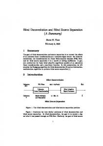
Mathematically, we can write the observed signals in source separation problem of instantaneous and linear mixtures as (see figure 1): n
(1)
ei (t ) = ∑ aij s j (t ) j =1
where A={ aij } is the mixing matrix. It is well known that such a system is invertible if the source signals are statistically independent and we have no more than one Gaussian signal. e1(t)
s1(t) s2(t)
y1(t) y2(t)
A
sn(t)
B
input
yn(t)
en(t) unknown (mixing system)
output
observation (demixing system)
Fig. 1. Block diagram of the mixture system and blind demixing system. Both matrix A and signals si(t) on the mixture process are unknown.
A solution may be found by minimizing the mutual information function between the outputs of the system yi:
n min B [I ( y )] = min B ∑ H ( yi ) − H (e ) − ln det (B ) i =1 A particular case of blind separation is the case of blind deconvolution, which is presented in figure 2, and can be expressed in the framework of Equation (1). Development of this framework is presented in the following section.
input
output
s(t)
e(t) h
unknown (convolution system)
y(t) w
observation (deconvolution system)
Fig. 2. Block diagram of the convolution system and blind deconvolution system. Both filter h and signal s(t) on the convolution process are unknown.
2 Model and assumptions We suppose that the input of the system S={s(t)}is an unknown non-Gaussian independent and identically distributed (i.i.d.) process. We are concerned by the restitution of s(t) observing the system’s output. This implies the blind inversion of a filter. From figure 2, we can write the output of filter h in a similar form that obtained in source separation problem, Equation 1, but now with vectors and matrix of infinite dimension:
e = Hs where: ... ... ... ... ... h (t + 1) ( ) ( − 1) h t h t H = ... h (t + 2 ) h (t + 1) h (t ) ... ... ... ...
... ... ... ...
is a Toeplitz matrix of infinite dimension and represents the action of filter h to the signal s(t). This matrix h is nonsingular provided that the filter h is invertible, i.e. -1 -1 -1 h exists and satisfies h ∗h = h∗h = δ0, where δ0 is de Dirac impulse. The solution to invert this systems and the more general nonlinear systems (Wiener systems) are presented and studied in [10, 11] where a Quasi-nonparametric method is presented. 2.1 Summary of the deconvolution algorithm From figure 2 we can write the mutual information of the output of the filter w using the notion of entropy rates of stochastic processes [12] as:
1 T ∑ H ( y (t ))− H ( y −T ,..., y T ) T → ∞ 2T + 1 t = − T
I (Y )= lim
(2)
= H ( y (τ )) − H (Y )
where τ is arbitrary due to the stationary assumption. The input signal S={s(t)} is an unknown non-Gaussian i.i.d. process, Y={y(t)} is the output process and y denotes a vector of infinite dimension whose t-th entry is y(t). We shall notice that I(Y) is always positive and vanishes when Y is i.i.d. After some algebra, Equation (2) can be rewritten as [10]:
I (Y )= H ( y (τ )) −
1 2π
2π
∫ log 0
+∞
∑ w(t )e
t = −∞
− jtθ
dθ − E [ε ]
(3)
To derive the optimization algorithm we need the derivative of I(Y) with respect to the coefficients of w filter. For the first term of Equation (3) we have:
∂H ( y (τ )) ∂w (t )
∂y (τ ) = −E ψ y ( y (τ )) = − E e (τ − t )ψ y ( y (τ )) ∂w (t )
(4)
where ψy(u)=(logPy)’(u) is the score function. The second term is:
∂ 1 ∂w(t ) 2π
2π
∫ log 0
+∞
∑
n =−∞
w ( n ) e − jnθ dθ =
1 2π
2π
∫ 0
e − jtθ +∞
∑ w (n ) e
− jnθ
dθ
(5)
n =−∞
where one recognizes the {−t}-th coefficient of the inverse of the filter w, which we denote w( −t ) . Combining Equations (5) and (6) leads to:
∂I (Y ) = − E x(τ − t )ψ y ( y (τ )) − w (− t ) ∂w(t )
[
]
that is the gradient of I(Y) with respect to w(t). Using the concept of natural or relative gradient, the gradient descendent algorithm will be finally as:
[
]
w ← w + µ {E x(τ − t )ψ y ( y(τ )) + δ }* w
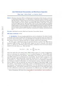
3 Application to speech signals If we want to apply this method to real word signals we have to solve the problem that the signals are usually not i.i.d., so we can not to use this method directly. In order to use that, we need to preprocess the input signal to ensure its temporal independence between samples and also to ensure its non-Gaussian distribution. 3.1 Whitening of speech signal For speech signals we observe that the i.i.d. condition is not attained and will be necessary a preprocessing stage consisting in a whitening of the original signal that can be done by an inverse LPC filter. In figure 3 we can see the autocorrelation sequence of a speech segment corresponding to the vowel /a/, before and after the whitening filter. Note that the prediction residual has peaks at multiples of the pitch frequency, and that the other periodicities are reduced.
Figure 3. Left: wave form of Vowel /a/ and thre prediction residual. Right: Comparison of the normalized autocorrelations of the vowel signal and the residual of the LPC.
The result obtained by a whitening filter is an i.i.d. signal but of Gaussian distribution because the output (error) signal in a linear predictors is Gaussian. Consequently it will be necessary to change de probability density function of the i.i.d. signal in order to acquire the necessary conditions to apply the deconvolution process in reception. 3.1 Des-Gaussianity of speech signal In figure 4 we show the quantiles of the signal and the residual vs. the quantiles of a gausian distribution. One can see that the whitened signal has a nearly linear relation and is simetric. In order to change its probability density function, we propose a method based on the following observations: 1.
Speech signals are periodic signals, with a fundamental period (frequency).
2.
A whitening filter removes all the components and keeps only the nonpredictable part that corresponds precisely to the excitation of the speech signal, the pitch, but the residual continues to be gausian distributed.
Starting from this observations we propose the following method for speech signals: 1.
Normalize the whitened signal provided by a LPC filter in a way that the maximums associated whit the periodic excitation been around ±1.
2.
Pass the result signal trough a nonlinear function that maintain the peak values but modify substantially all the other values, therefore the pdf. For this function we propose:
2.1. exponential function x(·)n: attenuate all the values between two consecutive peaks. 2.2. tanh(·): amplify all the values between two consecutive peaks.
Fig. 4. Plot of the quantiles of the whitened speech signal versus probability of a Gaussian. One can observe the Gaussianity of the distribution.
The effect of this process will be that the output signal will maintain important parts of the signal (the peaks of the series) and will change the form of the distribution. In the next figure we can see the proposed method:
s’(t)
s(t) M
k (.)
Preprocessing stage Fig. 5. The proposed preprocessing stage, composed by a whitening filter M and a nonlinear function k(·) preserving the most important part of the input signal.
4 Experimental results The input signal is a fragment of speech signal, preprocessed previously as scheme of figure 5. This is the signal that we want to transmit through an unknown channel. Our objective is to recover the original signal s’(t) only from the received observation e(t).
observed signal
input signal s’(t)
s(t) M
k (.)
convolution system (channel)
Preprocessing stage
observed signal e(t)
e(t) h
output signal s’’(t)
y’(t) w
blind deconvolution system
M
-1
Postprocessing stage
Fig. 6. On the top, the proposed preprocessing stage, and the convolution system. On the down, the blind deconvolution system and the postprocessing stage.
Consider, now, the filter h as a FIR filter with coefficients: h=[0.826,0.165,0.851,0.165,0.810]. Figure 7 shows that h has two zeros outside the unit circle, which indicates that h is non-minimum phase. The system that we propose will always yield a stable equalizer because it computes a FIR aproximation of the IIR optimal solution. The algorithm was provided with a signal of size T = 500. The size of the impulse response of w was set to 81. In the preprocessing stage the length of LPC was fixed at 12 coefficients and nonlinear function (des-Gaussianity) was k(u)=u3. In figure 8, at the left we show the prediction residual, before and after a cubic non-linearity. At the right we show a quantile plot of the residual vs. a gausian distribution. It can be seen that it does not follow a linear relation. The results showed in figure 9 prove the good behavior of the proposed algorithm, i.e. we perform correctly the blind inversion of the filter (channel). The recovered signal at the output of the system has the spectrum showed in figure 10. We can see how, although we have modified in a nonlinear manner the input signal in the preprocess stage, the spectrum matches the original because non-linear function k(·) preserve the structure of the residual (non-predictable part) of the signal. The difference between harmonic peaks of speech signal and background noise is about 40 dB so possibly this noise will not be heard due to the 'masking' effect.
Fig. 7. Zeros of h. We observe two zeros outside the unit circle, so the filter is of non-minimum phase.
Fig. 8. On the left, the lpc residue of the signal supperposed with the residual after the nonlinear opperation. On the right, the quantile of the processed residual versus the quantiles of a gausian distribution.
5. Summary In this paper we have presented a method for blind deconvolution of channel applied to real world signals, based on source separation techniques. These techniques assure that a channel is invertible if the original signal is non-Gaussian and i.i.d. In order to apply this result to speech signals we will need to preprocess the original signal due to its periodic characteristic (no i.i.d. property). To avoid this problem we propose a
whitening stage by means of an inverse LPC filter and applying after a non-linear function for des-Gaussianity the signal. This function should preserve the important part of the signal. Thereby we modify the density probability function without changing the important part of the signal. In reception, after the deconvolution of the signal, we need a postprocessing stage to obtain the original speech signal, by means of the LPC filter.
Fig. 9. In the left, filter coefficients evolution of the inverse filter w. The convergence is attained at 150 iterations approx. In the right, convolution between filter h and it's estimated inverse w. The result is clearly a delta function.
Fig. 10. Input signal spectrum (continuous line), output signal spectrum (dotted line) and LPC spectrum (Thick line). We can observe the similarity of these spectrums at low frequencies. The main difference is related to the high part of the spectrum of the reconstructed signal, which is due to the fact that the lpc recostruction alocates resources to the parts of the spectrum with high energies
For a future works we are studying other possibilities in order to apply source separation techniques to linear or non-linear channel deconvolution problems with real world signals. Our preliminary work indicated that we can effectively invert the
nonlinear deconvolution by means of source separation techniques [10, 11] but for a real word signals it is necessary to study how we can preprocess this signals to insure the i.i.d. and non Gaussian distribution necessary conditions to apply these techniques.
6. Acknowledgment This work has been in part supported by the University of Vic under de grant R0912 and by the Spanish CICyT project ALIADO.
References 1. Jutten, C., Hérault, J. ,“Blind separation of sources, Part I: An adaptive algorithm based on neuromimetic architecture”, Signal Processing 24, 1991. 2. Comon, P., “Independent component analysis, a new concept?”, Signal Processing 36, 1994. 3. Amari, S., Cichocki A., Yang, H.H., “A new learning algorithm for blind signal separation”, NIPS 95, MIT Press, 8, 1996 4. Comon, P., “Separation of sources using higher order cumulants” Advanced Algorithms and Architectures for Signal Processing, 1989. 5. Cardoso, J.P., “Source separation using higher order moments”, in Proc. ICASSP, 1989. 6. Puntonet, C., Mansour A., Jutten C., “A geometrical algorithm for blind separation of sources”, GRETSI, 1995 7. Bell, A.J., Sejnowski T.J., “An information-maximization approach to blind separation and blind deconvolution”, Neural Computation 7, 1995. 8. Nguyen Thi, H.L., Jutten, C., “Blind source separation for convolutive mixtures”, IEEE Transactions on Signal Processing, vol. 45, 2, 1995. 9. Taleb, A., Jutten, C., “ Nonlinear source separation: the post-nonlinear mixtures”, in Proc. ESANN, 1997 10. Taleb, A., Solé, J., Jutten, C., “Blind Inversion of Wiener Systems”, in Proc. IWANN, 1999 11. Taleb, A., Solé, J., Jutten, C., “Quasi-Nonparametric Blind Inversion of Wiener Systems”, IEEE Transactions on Signal Processing, 49, n°5, pp.917-924, 2001 12. Cover, T.M., Thomas, J.A., Elements of Information Theory. Wiley Series in Telecommunications, 1991.