1750
IEEE TRANSACTIONS ON NEURAL NETWORKS, VOL. 18, NO. 6, NOVEMBER 2007
Block-Based Neural Networks for Personalized ECG Signal Classification Wei Jiang, Student Member, IEEE, and Seong G. Kong, Senior Member, IEEE
Abstract—This paper presents evolvable block-based neural networks (BbNNs) for personalized ECG heartbeat pattern classification. A BbNN consists of a 2-D array of modular component NNs with flexible structures and internal configurations that can be implemented using reconfigurable digital hardware such as field-programmable gate arrays (FPGAs). Signal flow between the blocks determines the internal configuration of a block as well as the overall structure of the BbNN. Network structure and the weights are optimized using local gradient-based search and evolutionary operators with the rates changing adaptively according to their effectiveness in the previous evolution period. Such adaptive operator rate update scheme ensures higher fitness on average compared to predetermined fixed operator rates. The Hermite transform coefficients and the time interval between two neighboring R-peaks of ECG signals are used as inputs to the BbNN. A BbNN optimized with the proposed evolutionary algorithm (EA) makes a personalized heartbeat pattern classifier that copes with changing operating environments caused by individual difference and time-varying characteristics of ECG signals. Simulation results using the Massachusetts Institute of Technology/Beth Israel Hospital (MIT-BIH) arrhythmia database demonstrate high average detection accuracies of ventricular ectopic beats (98.1%) and supraventricular ectopic beats (96.6%) patterns for heartbeat monitoring, being a significant improvement over previously reported electrocardiogram (ECG) classification results. Index Terms—Block-based neural networks (BbNNs), evolutionary algorithms (EAs), personalized electrocardiogram (ECG) classification.
I. INTRODUCTION LECTROCARDIOGRAM (ECG) is an important routine clinical practice for continuous monitoring of cardiac activities. However, ECG signals vary greatly for different individuals and within patient groups [1]. Even for the same individual, heartbeat patterns significantly change with time and under different physical conditions. While normal sinus rhythm originates from the sinus node of heart, arrhythmias have various origins and indicate a wide variety of heart problems. Under different situations, the same symptoms of arrhythmia produce different morphologies due to their origins such as premature
E
Manuscript received April 11, 2006; revised October 5, 2006 and February 24, 2007; accepted March 25, 2007. This work was supported by the National Science Foundation under Grant ECS-0319002. W. Jiang is with the Department of Electrical and Computer Engineering, The University of Tennessee, Knoxville, TN 37996-2100 USA (e-mail: wjiang@utk. edu). S. G. Kong is with the Department of Electrical and Computer Engineering, Temple University, Philadelphia, PA 19122 USA (e-mail:
[email protected]). Color versions of one or more of the figures in this paper are available online at http://ieeexplore.ieee.org. Digital Object Identifier 10.1109/TNN.2007.900239
ventricular contraction [2], [3]. Association for the Advancement of Medical Instrumentation (AAMI, Arlington, VA) recommends that each heartbeat be classified into one of the fol(beats originating in the sinus lowing five ECG patterns: node), (supraventricular ectopic beats), (ventricular ectopic beats), (fusion beats), and (unclassifiable beats) for heart monitoring [4], [5]. A number of methods have been proposed to classify ECG heartbeat patterns based on the features extracted from ECG signals, such as morphological features [5], heartbeat temporal intervals [5], frequency domain features [3], [6], and wavelet transform coefficients [7]. Classification techniques for ECG patterns include linear discriminant analysis [5], support vector machines [8], artificial neural networks (NNs) [9]–[14], mixture-of-experts method [12], and statistical Markov models [15], [16]. Unsupervised clustering of ECG complexes using self-organizing maps has also been studied [17]. Many conventional supervised ECG classification methods based on fixed classification models [5], [8], [15], [16] or fixed network structures [9]–[11] do not take into account physiological variations in ECG patterns caused by temporal, personal, or environmental differences. Evolvable NNs [18] change the network structure and internal configurations as well as the parameters to cope with dynamic operating environments. Block-based neural network (BbNN) models [19] provide a unified approach to the two fundamental problems of artificial NN design: simultaneous optimization of structures and weights and implementation using reconfigurable digital hardware. An integrated representation of network structure and connection weights of BbNNs offers simultaneous optimization by use of evolutionary optimization algorithms. BbNNs have a modular structure suitable for implementation using reconfigurable digital hardware. The network can be easily expanded in size by adding more blocks. A BbNN can be implemented using field-programmable gate arrays (FPGAs) that can modify and fine-tune its internal structure “on the fly” during the evolutionary optimization procedure. A library-based approach [20] creates a library of VHSIC hardware description language (VHDL) modules of the basic BbNN blocks and interconnects the modules to form a custom BbNN network, which is then synthesized, placed and routed, and downloaded to an FPGA. A more recent effort [21] proposes a “smart block” to implement a basic block of any input/output type with an Amirix AP130 board that features a Xilinx Virtex-II Pro FPGA, dual on-chip PowerPC 405 processors, and on-chip block random access memories (BRAMs). This approach is a system-on-chip design with an evolutionary algorithm (EA) running on PowerPC and a BbNN network implemented on the FPGA. Research work [22], [23] has been
1045-9227/$25.00 © 2007 IEEE
JIANG AND KONG: BBNNS FOR PERSONALIZED ECG SIGNAL CLASSIFICATION
carried out to implement a complete EA on FPGAs that results in performance improvement over software implementation. This paper presents BbNNs for personalized ECG heartbeat pattern classification that evolve the structure and the weights for different individuals. Classifiers with a fixed structure and parameters trained with a training set often fail to trace large variations in ECG signals. Earlier work on BbNN classifiers for ECG signal analysis have demonstrated a potential for performance improvement over conventional techniques [24], [25]. Personalized ECG signal classification aims at reconfiguration of the structure and parameters to compensate the variations in ECG patterns caused by temporal, individual, and environmental differences. In this paper, only the variations in personal differences are considered. Both structure and internal weights of a BbNN classifier are evolved specifically for an individual patient using patient-specific training data. A feedforward network configuration is used to facilitate hardware implementation with less hardware resources and enable the use of gradient-based local search for weight optimization. The gradient-based local search speeds up the slow convergence of conventional evolutionary optimization schemes. A fitness scaling with generalized disruptive pressure that favors individuals of high and low fitness values reduces the possibility of premature convergence. An adaptive rate update scheme automatically adjusts the operator rates by rewarding or penalizing an operator based on the effectiveness in the previous evolution steps. The adaptive rate update enhances the fitness trend compared to predetermined fixed operator rates. The Hermite transform coefficients and a time interval between the two neighboring R-peaks of an ECG waveform are used as the inputs to the network. The network structure and weights of a selected BbNN are evolved for a patient using both common and patient-specific training patterns to provide personalized heartbeat classification. Simulation results using the Massachusetts Institute of Technology/Beth Israel Hospital (MIT-BIH) arrhythmia database demonstrate high average accuracies of 98.1% and 96.6% for the detection of ventricular ectopic beats (VEBs) and supraventricular ectopic beats (SVEBs), which presents a significant improvement over previously published ECG classification results. The proposed method is compared with two popular methods for ECG classification using the MIT-BIH database. Automatic heartbeat classification [5] based on linear discriminant uses various sets of morphology and heartbeat interval features. An NN-based method [12] distinguishes VEB from non-VEB beats using a mixture-of-experts approach. BbNNs implemented in FPGAs facilitate “on-the-fly” reconfiguration of network parameters for personalized ECG signal classification. The remainder of this paper is organized as follows. Section II reviews the basic concepts and the properties of BbNNs as a general computing platform. Section III describes an evolutionary optimization scheme that includes fitness scaling with generalized disruptive pressure, evolutionary and gradient-based search operators, and an adaptive rate update scheme. Section IV details the Hermite transform for feature extraction of ECG signals, fitness function, and the classification results of ECG heartbeat patterns using the MIT-BIH arrhythmia database. Section V concludes the paper.
1751
Fig. 1. Structure of BbNNs.
II. BBNNS A BbNN can be represented by a 2-D array of blocks. Each block is a basic processing element that corresponds to a feedforward NN with four variable input/output nodes. A block is connected to its four neighboring blocks with signal flow represented by an incoming or outgoing arrow between the blocks. Signal flow uniquely specifies the internal configuration of a block as well as the overall network structure. Fig. 1 BbNN with illustrates the network structure of an rows and columns of blocks labeled as . The first row is the input layer and the blocks of blocks form the output layer. BbNNs with columns can have up to inputs and outputs. Redundant input nodes take a constant input value, and the output nodes not used are ignored. An input signal propagates through the blocks to produce network output . Due to its modular characteristics, a BbNN can be easily expanded to build a larger scale network. The size of a BbNN is only limited by the capacity of reconfigurable hardware used. A feedforward network configuration with all downward vertical signal flows is used in this paper to facilitate hardware implementation of BbNNs. A feedback configuration of BbNN architecture may cause a longer signal propagation delay to produce an output. Also, the need to store the network states in feedback implementation tends to require extra hardware resources. Feedforward implementation enables the use of gradient-based local search that can be combined with evolutionary operators to increase the convergence speed of evolutionary optimization. A block can be represented by one of the three different types of internal configurations. Fig. 2 shows three types of internal configurations of one input and three outputs (1/3), three inputs and an output (3/1), and two inputs and two outputs (2/2). The four nodes inside a block are connected with each other through denotes a connection from node to node weights. A weight . A block can have up to six connection weights including the
1752
IEEE TRANSACTIONS ON NEURAL NETWORKS, VOL. 18, NO. 6, NOVEMBER 2007
Fig. 2. Three possible internal configuration types of a block. (a) One input and three outputs (1/3). (b) Three inputs and one output (3/1). (c) Two inputs and two outputs (2/2).
biases. For the case of two inputs and two outputs (2/2), there are four weights and two biases. The 1/3 case has three weights and three biases, and the 3/1 three weights and one bias. Internal configuration of a BbNN is characterized by the input/output connections of the nodes. A node can be an input or an output according to the internal configuration determined by the signal flow. An incoming arrow to a block specifies the node as an input, and output nodes are associated with outgoing arrows. Generalization capability of BbNN emerges through various internal configurations of a block. The signal denotes the input and the output of the block. The output of a block is computed with an activation function Fig. 3. EA for BbNN optimization.
(1) and are index sets for input and output nodes. For type 1/3 and . For blocks of the type 3/1, block, and . The type 2/2 blocks have and . The term is the bias of the th node. In this paper, a sigmoid activation function of the form (2) and [26]. These parameters is used with were chosen so that the first derivative at zero approximately equals 1, the second derivative achieves its extremum at approximately 2 and 2, and its linear range is 1, 1. III. EVOLUTIONARY OPTIMIZATION OF BBNN A. EA for BbNN Optimization Evolutionary optimization of BbNN involves four main procedures: fitness scaling, selection, evolutionary and gradient search operations, and adaptive operator rate adjustment. The fitness is rescaled with a generalized disruptive pressure that favors the individuals with both high and low fitness values. A tournament selection chooses parent individuals into a mating pool subject to crossover, mutation, and gradient-based local search operations. The rate of an operator is updated adaptively in terms of the effectiveness of the operator in generating fitter individuals. Fig. 3 shows a pseudocode description of the evolutionary optimization algorithm. After a random generation of initial pop-
ulation, the algorithm enters into the evolution loop. The current population is evaluated to update individual fitness values. The fitness rescaling by disruptive pressure ensures the selection of some individuals with high and low fitness values. Initially, each operator is selected according to a uniform distribution. Applying this operator according to its rate to the parent(s) chosen with tournament selection produces new offspring. This offspring is reinserted into the population and replaces an inferior individual chosen with a tournament selection. The evoluof generations tion process during a predetermined number is called an evolution period. After each evolution period, the operator rates are updated based on their effectiveness. The EA is terminated either by finding a satisfactory solution or after the maximum generation is reached. Two successive populations differ by a single individual in this incremental EA [27], [28]. In generational EA models, a new population replaces the old population. An incremental EA is preferred over the generational model in order to reduce the computational and memory requirements at each generation. B. Fitness Scaling and Tournament Selection In many optimization problems, the search landscape can be rather mountainous or multipeaked. The search space of BbNNs resembles a mountainous characteristic due to the two reasons. First, each of the possible structures will lead to a local optimum if the weights are properly optimized. Second, for a given structure, the weight space can also contain many peaks. In the “needle-in-a-haystack” problem, the global optimum is sur-
JIANG AND KONG: BBNNS FOR PERSONALIZED ECG SIGNAL CLASSIFICATION
Fig. 4. Fitness scaling with a generalized disruptive pressure.
rounded by poor solutions and isolated from other good regions. The proportional selection that favors good individuals was criticized for its inefficiency in finding the global optimum for such problems [29], [30]. A selection scheme with disruptive pressure devotes more trials to both superior and inferior individuals and helps improve search performance as one of the solutions to such problems [29]. A popular disruptive pressure method modifies the actual fitness by taking an absolute difference of the [30] fitness with the average fitness value (3) denotes the fitness function rescaled with disruptive where pressure. In this paper, a modified fitness scaling function with generalized disruptive pressure is used, which is more flexible with the original scheme included as a special case. The fitness funcand the average tion is rescaled using the minimum fitness fitness (4) The scaling function adjusts the degree of selecting an individual whose fitness is near the minimum by controlling the parameter that adjusts the degree of disruptive pressure in the range of . For , the scaling function becomes a linear function with no disruptive pressure. When , the fitness function becomes the usual disruptive presas in (3). In this paper, was sure that centers at used. Fig. 4 shows the relationship between the fitness and the new fitness rescaled with the generalized disruptive pressure. and have a linear relationship with a discontinuity at . The fitness scaling function scales the fitness to the range between 0 and . As evolution procedure proceeds, the average fitness tends to come . The fitness scaling method with near the maximum fitness the modified disruptive pressure assures that the bending point and , which is located between the two fitness values prevents the superior individuals from being rescaled to low fitness values as the original scheme does. Two selection processes are present in the EA: parent selection for evolutionary and local search operations and survivor selection for reinsertion [28]. Parent selection picks one or a pair of individuals from the old population for variation operation. A roulette-wheel selection finds individuals in proportional to the fitness value. Despite its popularity,
1753
roulette-wheel selection may have problems such as premature convergence in early phase of evolution or genetic drift in later phase of evolution. Tournament selection picks out the best one from randomly chosen individuals [31]. Tournament selection has the same effects as both fitness proportional sampling and selection probability adjustment [32], [33]. It has the useful property of not requiring global knowledge of the population. The tournament size closely adjusts the selection pressure. A larger tournament size imposes a higher selection pressure. Binary tournament used in this paper for parent selection finds the better individual of the two selected randomly, i.e., . Survivor selection determines which member of the current population is to be replaced with the newly produced offspring. The commonly used scheme of replacing the worst implements an elitism strategy that keeps the best trait found so far. However, it is likely to cause premature convergence, because an outstanding individual can quickly take over the entire population under such a scheme [28]. In this paper, a tournament selection that picks the worst individual among five randomly selected individuals is used. C. Evolutionary Operators With Adaptive Rate Update 1) Crossover: Crossover and mutation serve as basic genetic operators used to evolve the structure and weights of BbNNs. For crossover operation of a pair of BbNNs, a group of signal flows are randomly selected. The selected signal flows are exchanged according to the crossover rate. After the exchange, the internal structure of a block is reconfigured according to the new signal flows. As a result, some weights in a BbNN will have corresponding weights in the other BbNN and some will not. Each of the corresponding weights will be updated by a weighted combination as in (5). The weights with no correspondences remain unchanged. Crossover operation can be done in two steps: signal flow and connection weights. Fig. 5 shows an example of crossover operation. For two individual BbNNs, signal flows of the same location are exchanged. Fig. 5(a) and (b) demonstrates two individual BbNNs before the crossover operation. Three , and are randomly selected for basic blocks crossover. Two individual BbNNs in Fig. 5(c) and (d) are after the crossover operation. Internal configurations of the blocks are rearranged after the crossover. Crossover operation of a pair of BbNNs takes the following manipulations. 1) Randomly select signal flows to be crossed over. 2) Identify the blocks and the connection weights of the blocks that are connected to the signal flows. Crossover operation can be done for the following two cases. a) When the signal flow remains unchanged after crossover and from the Take two corresponding weights two blocks. The crossover operation for real-valued weights is defined as
(5) where
denotes a uniform random number in
.
1754
Fig. 5. Crossover operation example of two 3
IEEE TRANSACTIONS ON NEURAL NETWORKS, VOL. 18, NO. 6, NOVEMBER 2007
2 4 BbNNs. A pair of individual BbNNs (a) and (b) before crossover and (c) and (d) after crossover.
b) When the signal flow changes after crossover Changed signal flow modifies internal configuration of the block. New connection weights generated accordingly are initialized with Gaussian random numbers having zero mean and unit variance, while not connected weights are removed. Fig. 6 shows an example of crossover when the signal flow changes after crossover. In Fig. 6(a), the signal flow bit between the blocks indicates a leftward connection. The two connection weights that are connected to this signal flow are represented as dotted arrows. Assuming that the signal flow is flipped after the crossover of the signal flows, the internal configurations of the two blocks will be updated as in Fig. 6(b), where the weights connected to the changed signal flow are represented in dotted arrows. Changing the signal flow will affect several connection weights of the two neighboring blocks. Newly generated weights are randomly initialized. Inactive weights are not used in the crossover operation. The proposed crossover operator has an advantage that the network structure and connection weights can be optimized at the same time. In early stage of learning, BbNN individuals have a variety of network structures. As the evolution process proceeds, a small number of possible structures tend to survive. As a result, crossover for signal flow will not change internal configurations as well as structure. Therefore, the optimization task will be mostly weight optimization in later stages of evolution.
Fig. 6. Internal configuration due to changing signal flow (a) before and (b) after crossover.
2) Mutation: Mutation operator randomly adds a perturbation to an individual according to the mutation rate. A BbNN has different mutation rates for the structure bit string and the weights. Structure mutation refers to an operation that flips a signal flow according to the structure mutation rate. When signal
JIANG AND KONG: BBNNS FOR PERSONALIZED ECG SIGNAL CLASSIFICATION
1755
flow is reversed after mutation, all the irrelevant weights are removed and new weights are created with random values in a proper direction. A weight selected for mutation will be updated with a random perturbation
is the sensitivity of the output node of the block in where that is connected to the current output node via . stage Thus, the weight update can be summarized in the following equation using (10)–(12):
(6)
(13)
where denotes zero-mean unit-variance Gaussian noise. 3) Gradient–Descent Search: The gradient–descent search (GDS) operator updates internal weights in a BbNN. A GDS epoch consists of forward pass to compute network outputs and a backward pass of error signals to update internal weights. The computation stage of a block determines the computational priority of the block
The sensitivities of the output nodes of the blocks in calculation stage are calculated, and then, the internal weights of given in these blocks are updated by adding the increment (13). After calculating the sensitivities and updating the weights of all blocks in stage , the sensitivities of the output nodes of the blocks in stage are computed with the weights update followed. This procedure continues until the calculation of the blocks in the first computation stage is finished. The GDS operation stops when either a preset maximum number of epochs are reached or the fitness improvement between two successive epochs falls below a threshold. The maximum number of epochs or a small threshold ensure a reasonable amount of computation at each generation. 4) Operator Rate Update: An operator rate determines the probability of the operator to be applied. The proposed update scheme automatically adjusts an operator’s rate based on both its effectiveness in improving the fitness in the previous step and current fitness trend. Operator rates are updated at every evolution period and remain unchanged during each evolution th evolution period, the first step is to assign period. In the a probability to each of the operators based on its performance during the th period. Then, the operator rates are increased if the maximum fitness has not been improved during the past period. The performance of an operator during the th evolution period is measured by the effectiveness defined as
(7) where denotes the computation stage of the blocks connected to the current block with outgoing signal flows. If a block does not receive input from the neighboring blocks, computation are stage becomes 1. The inputs to the blocks in stage updated with the outputs of the blocks in stage , followed by . This forward computing the outputs of the blocks in stage pass is complete when the network output is obtained. In a backward pass, the error signals propagate from the blocks of higher stages to lower stages. The error criterion function is defined as (8) is the total number of training patterns. The two vecwhere tors and are the target and actual outputs for the th training pattern, respectively. Gradient steepest descent rule updates the weights according to the following equation [34]: (9) where is the learning rate. and are the index sets of input of the internal weight of and output nodes. The increment a block can be deduced using generalized delta rule [35], [36] (10) where is the sensitivity of the output node of the block to the error, and is the input to the input node of the block. For a network output node, the sensitivity becomes (11) where and are the desired and actual outputs at the node. is the first derivative of the tangent activation function and is a net input to the node. The sensitivity of an output node of a block in stage is computed as (12)
(14) denotes the number of generations within each evowhere lution period that an operator produces offspring with higher indicates the total fitness value than that of its parents, and number of generations that an operator is selected in the same has a range from 0 (least evolution period. Thus, the value of effective) to 1 (most effective). The effectiveness of an operator , determines its probability in the next evolution period as defined in the following: if if (15) where is a scaling factor that controls the amount of rate adjustment and has been set to 0.02 randomly for initial simulaand denote lower and upper limits of the probtions. , the operator ability for an operator to be applied. If will never be applied, and if , then the operator will is set to a big value (e.g., 1.0) always be applied. Initially, to ensure an effective operator to be applied with a higher rate is set to a small value (e.g., 0.1) to give “less effecand tive” operators a lower chance being applied. Overall, the update scheme uses high operator rates in early evolution stages, and then, gradually decreases the rates for less effective operators.
1756
IEEE TRANSACTIONS ON NEURAL NETWORKS, VOL. 18, NO. 6, NOVEMBER 2007
Effective operators keep higher rates. The logarithmic function is used in the rate update scheme to implement gradual rate adjustment. The next step in rate adjustment considers the fitness trend during the previous evolution periods. The algorithm tends to fall in a local maximum point if the maximum fitness stops improving before a desired solution is found. It is thus desired to perform more searches in order to help the search escape from a local solution, and the operator rates are accordingly increased to consider such situation as described in the following:
if
Fitness
(16)
is the set slightly bigger than to ensure the rate is where increased ( equals 5% percent bigger than in the experimeans the maximum fitness has ments). Fitness not been improved during the th evolution period. An operator rate is determined according to the performance and the current fitness trend. An operator will maintain a high rate if it is effective in generating fitter individuals; otherwise, its rate will be gradually decreased. If the maximum fitness has not been improved before a desired solution was found, the operator rates will be increased to do denser searches. IV. ECG SIGNAL CLASSIFICATION The AAMI recommends that each ECG beat be classified into (beats originating in the the following five heartbeat types: sinus node), (supraventricular ectopic beats), (ventricular ectopic beats), (fusion beats), and (unclassifiable beats) [4]. A large interindividual variation of ECG waveforms is observed among individuals and within patient groups [1]. The waveforms of ECG beats from the same class may differ significantly and different types of heartbeats sometime possess similar shapes. Hence, the sensitivity and specificity of ECG classification algorithms are often unsatisfactorily low. For instance, a recent method [5] reports a sensitivity rate of 77.7% for VEB detection and 75.9% for SVEB detection. A. ECG Data The MIT-BIH arrhythmia database [2] is used in the experiment. The database contains 48 records obtained from 47 different individuals (two records came from the same patient). Each record contains two-channel ECG signals measured for 30 min. Twenty-three records (numbered from 100 to 124, inclusive with some numbers missing) serve as representative samples of routine clinical recordings. The remaining 25 (numbered from 200 to 234, inclusive with some numbers missing) records include unusual heartbeat waveforms such as complex ventricular, junctional, and supraventricular arrhythmias. Continuous ECG signals are filtered using a bandpass filter with a passband from 0.1 to 100 Hz. Filtered signals are then digitized at 360 Hz. The beat locations are automatically labeled at first and verified later by independent experts to reach a consensus. The whole database contains more than 109 000 annotations of normal and 14 different types of abnormal heartbeats.
The normal and various abnormal types have been combined into five heartbeat classes according to the AAMI recommended practice [4]. In earlier work [25], a binary classification of VEB and non-VEB problem was addressed. Paced beats refer to ECG signals generated by the heart under the help of an external or implanted artificial pacemaker for the patients whose electrical conduction path of heart is blocked or the native pacemaker is not functioning properly. In agreement with the AAMI-recommended practice, paced beats are not included in the classification experiments in this paper as well as in the previous works [5], [12] chosen for comparison. The remaining records are divided into two sets. The first set contains the 20 records numbered from 100 to 124 and is intended to provide common representative training data. The second set is composed of the rest records numbered from 200 to 234, and each of the records in this set will be used in the test for performance evaluation. The training data for a patient consist of two parts, the first part coming from the common set and being the same for all testing patients. The other part includes the heartbeats from the first 5 min of the ECG recording of the patient, which conforms to the AAMI recommended practice that allows at most 5 min of recordings from a subject to be used for training purpose. The remaining beats of the record are test patterns. B. Feature Extraction Basis function representations have been shown to be an efficient feature extraction method for ECG signals [37], [38]. Hermite basis functions provide an effective approach for characterizing ECG heartbeats and have been widely used in ECG signal classification [8], [9], [17] and compression [37]. Hermite basis function expansion has a unique width parameter that is an effective parameter to represent ECG beats with different QRS complex duration. The coefficients of Hermite expansions characterize the shape of QRS complexes and serve as input features. Hermite basis functions are given by the following: (17) where is the width parameter and approximately equals the are the Hermite half-power duration. The functions polynomials [9], [17]. Hermite functions are orthonormal for any fixed value of width (18) This useful property enables the calculation of expansion coefficients of an arbitrary signal. Specifically, the QRS complex is extracted as a 250-ms window centered at the R-peak, which is sufficient to cover both normal and wider-than-normal QRS can be approximated by signals [9], [39]. A QRS complex a combination of Hermite basis functions weighted by expansion coefficients (19) as . Multiplying to both where sides of (19) and summing them up over time, a set of coef-
JIANG AND KONG: BBNNS FOR PERSONALIZED ECG SIGNAL CLASSIFICATION
ficients are obtained by applying the orthonormal property in (18)
(20) Clearly, the expansion coefficient depends on the width . To minimize the summed square error between the actual and approximated complex for a given , the parameter is increased stepwise to its upper bound determined using the algorithm described in [17]. Different numbers of expansion coefficients can be used to approximate a QRS complex. The approximation error depends on the number of coefficients. There is a tradeoff between approximation error and computation time. More coefficients lead to smaller errors, but result in heavy computation burden. Furthermore, a small number of coefficients are able to approximate the heartbeats with small representation errors. Five Hermite functions allow a good representation of the QRS complexes and fast computation of the coefficients [17]. Besides the basis function coefficients and width parameter , the time interval between two neighboring R-peaks is included to discriminate normal and premature heart beats. C. Fitness Function Fitness function evaluates the quality of the solutions found by EAs. The fitness of an individual BbNN is defined as Fitness
(21) and are the numbers of samples in the common where denotes the and patient-specific training data, respectively. number of output blocks. controls relative importance of the common and patient-specific training in the final fitness , and a small value less than 0.5 (0.2 in this paper) gives more weight for correctly classifying patient-specific patterns. Both common and patient-specific training patterns are considered in the fitness function. While patient-specific data may serve as the training data for evolving BbNN specific to a patient, the inclusion of common training data is useful when the small segment of patient-specific samples contains few arrhythmia patterns [2]. To construct the common data set, representative beats from each class are randomly sampled. Since the number of normal beats is as high as ten times more than the other beat types [2], no type- beats are selected, but 5% of type- (64), 30% of type- (58), and all type- (13) and type- (7) beats are included to have the total 142 beats in the common set. The number of beats in the patient-specific training data varies due to the difference in the heart rates of different patients.
1757
D. Experiment Results 1) Training Parameters: In BbNNs, the number of columns is equal to or greater than the number of input features. The number of rows needs to be determined so that the network has sufficient complexity for a given problem. A small network size is preferred, provided that it achieves the desired performance. Too big a network runs the risk of overfitting that causes poor generalization performance, and requires a more complex optimization process because of higher degree of freedom in the search space. In the experiment, a 2 7 network was selected as a minimum-size BbNN that can take seven input features. Population size affects the amount of time consumed in a generation. Though a large population size requires more com) contains puting resources, a small population size (e.g., few “building” patterns and, therefore, may take even longer evolution time to find a solution. The maximum fitness defines the quality of the desired solution. A high maximum fitness usually needs more generations and can lead to value an overfitted solution. A small GDS learning rate is necessary for the learning to converge. The EA parameters are selected to meet the constraints: population (80), stop generation (3000), , and maximum fitness (0.92), rate update interval learning rate for GDS . These parameters demonstrated fast convergence speed for initial simulations. The same set of parameters has been used for all test records without fine-tuning for specific patients. The desired output for the target category and nontarget categories are, respectively, set to and . 2) Evolution Trends: EAs are applied to evolve the selected BbNN for a patient. Fig. 7(a) shows a typical fitness trend. The dotted and solid line corresponds to the respective average and maximum fitness. The evolution stops when the desired fitness is met after approximately 2200 generations. Fig. 7(b) demonstrates structure evolution process in terms of the percentage of occurrences of different structures. A solid line indicates the occurrences of a near-optimal structure. The others represent four nonoptimal structures. The number of BbNNs with a near-optimal structure increases during the evolution and becomes dominant and relative stable in the population after about 800 generations. Fig. 8 demonstrates an operator rate update trend. The GDS rate is almost constant with some fluctuations through entire evolution process, while the crossover operator favors a higher rate with bigger fluctuations than that of the GDS. The rates for two mutation operators have similar trend that decreases slowly overall and increases sometimes, when fitter individuals are generated by the mutations or the fitness has not been improved [see Fig. 7(a)]. Fig. 9 shows the effect of the adaptive rate update scheme in terms of the convergence speed of maximum fitness. In the fixed rate case, the GDS and the crossover use a high rate (0.8) and the mutations use a low rate (0.2). The fitness trends are averaged over ten independent runs. Each error bar shows a standard deviation of the maximum fitness at every 200 generations. The error pattern for the fixed rate case is similar to that for the adaptive rate update scheme. The EA with adaptive rates achieves noticeably higher fitness value on average after the conventional evolution procedure. The fitness scaling also
1758
IEEE TRANSACTIONS ON NEURAL NETWORKS, VOL. 18, NO. 6, NOVEMBER 2007
Fig. 8. Adaptive operator rate adjustment scheme.
Fig. 7. (a) Fitness trend. (b) Percentage of occurrences of the structures with higher fitness values.
enhances fitness levels. The EA GDS algorithm without fitness scaling produces the mean and maximum fitness values of 0.900 and 0.909 in ten trials, which can be compared to 0.920 and 0.942 when the fitness scaling is applied. The GDS operator was tested in terms of convergence speed. Fig. 9 shows maximum fitness trend during the evolution procedure averaged over ten runs. The GDS operator quickly increases the fitness with relatively small error variations than the EA without GDS. The EA algorithm reaches its maximum fitness of 0.837 in 3000 generations, while the proposed EA with GDS algorithm (EA GDS) takes only 30 generations to reach the same level of fitness. This leads to a significant saving in computation time from 222.5 to 5.2 s in simulations with a typical Pentium IV PC. A BbNN classifier is evolved specifically for each patient. Both structure and internal weights of a BbNN are optimized with the EA. Fig. 10 shows the network structure of the BbNNs
Fig. 9. Comparison of maximum fitness trends for different evolutionary optimization settings.
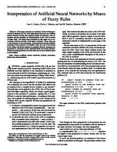
evolved from 24 patients. The numbers on the arrow are occurrence counts of the same signal flows among 24 individual BbNNs. The maximum output indicates the classified ECG type. The redundant output nodes are marked by . Inputs to the BbNN are the five Hermite transform coeffi. The input is the Hermite width and is cients the time interval between two neighboring R-peaks. 3) Classification Results: Table I summarizes classification results of ECG heartbeat patterns for test records. Two sets of performance are reported: the detection of VEBs and the detection of SVEBs, in accordance with the AAMI recommendations. Four performance measures, classification accuracy (Acc), sensitivity (Sen), specificity (Spe), and positive predictivity (PP), are defined in the following using true positive (TP), true negative (TN), false positive (FP) and false negative (FN). Classification accuracy is defined as the ratio of the number of correctly classified patterns (TP and TN) to the total number of patterns classified. Sensitivity is the correctly detected events
JIANG AND KONG: BBNNS FOR PERSONALIZED ECG SIGNAL CLASSIFICATION
1759
Fig. 10. BbNN structure evolved from 24 patients.
TABLE I SUMMARY OF BEAT-BY-BEAT CLASSIFICATION RESULTS FOR THE FIVE CLASSES RECOMMENDED BY THE AAMI
(VEB or SVEB) among the total number of events and is equal to TP divided by the sum of TP and FN. Specificity refers to the rate of correctly classified nonevents (non-VEBs or non-SVEBs) and is, therefore, the ratio of TN to the sum of TN and FP. Positive predictivity refers to the rate of correctly classified events in all detected events and is, therefore, the ratio of TP to the sum of TP and FP. The classification of ventricular or unknown beats as VEBs does not contribute fusion to the calculation of classification performance according to AAMI recommended practice. Similarly, performance calculation for detecting SVEBs does not consider the classification of unknown beats as SVEBs. Each experiment was performed ten times. The coefficient of variation (CV) measures dispersion of a probability distribution and is defined as the ratio of standard deviation to mean, which allows comparison of the variation of populations that have significantly different mean values. The CVs for true positive beats of , , , and types are 0.9%, 1.3%, 4.0%, and 48.3%, respectively. The variations for , , and types are small except type , which has a very small number of instances. For VEB detection, the sensitivity was 86.6%, the specificity was 99.3%, the positive predictivity was 93.3%, and the overall accuracy was 98.1%. For SVEB detection, the sensitivity was 50.6%, the specificity was 98.8%, the positive predictivity was 67.9%, and the overall accuracy was 96.6%. From the results, the performance of SVEB detection is not as good as VEB detection, and the possible reasons include the more diverse types in class and the lack of class training patterns in patients [2], [5]. The proposed technique is compared to earlier works using the AAMI standards. An automatic heartbeat classification
method [5] is based on linear discriminants and various sets of morphology and heartbeat interval features. The database was divided into two sets with each containing 22 recordings. The best classifier configuration determined using the first set was used to classify the heartbeats in the second set for performance evaluation. An NN method based on mixture-of-experts concept [12] distinguishes VEB from non-VEB beats. The algorithm employs a test set of 20 recordings that excluded records without premature ventricular contractions. A global expert was developed using both unsupervised self-organizing map and supervised learning vector quantization based on a common set of ECG training data. A local expert was developed similarly but based solely on patient-specific training data. The decisions from both classifiers are then linearly combined using coefficients from a gating network that is trained with another set of patient-specific ECG data. Fig. 11 shows the comparison results of the proposed method with the two methods in terms of VEB and SVEB detection. The comparison results of VEB detection are based on 11 recordings that are common to all the three studies. SVEB detection is based on 14 common recordings of the proposed method and [5], but not [12], since the work is limited to VEB detection. False positive rate (FPR) versus true positive rate (TPR) is marked as a receiver operating characteristics (ROC) curve [40]. and FPR ) correThe ideal classification case (TPR sponds to the upper left corner of the ROC curve. Therefore, a TPR-FPR combination is considered better as it is closer to the upper-left corner. The proposed method generates higher TPR but lower FPR compared to the other two methods. Table II summarizes sensitivity, specificity, positive predictivity, and overall accuracy of the three methods. The proposed method outperforms the other two methods for all the metrics used in VEB detection. For SVEB detection, the proposed method produces the sensitivity comparable to and higher specificity than [5]. There are other works in the literature that cannot be directly compared with the proposed method since they use a subset of the MIT-BIH database or aim at identifying specific ECG types. Hu et al. [11] proposed multilayer-perceptrons (MLP) network of the size 51-25-2 trained with backpropagation algorithm for the classification of normal and abnormal heartbeats with an average accuracy of 90% and 84.5% in classifying the beats into 13 beat types according to the MIT-BIH database annotations. In [3], the use of MLP and the Fourier transform features results in 2% of mean error for three rhythm types based on 700 test
1760
IEEE TRANSACTIONS ON NEURAL NETWORKS, VOL. 18, NO. 6, NOVEMBER 2007
utilizes evolutionary and gradient-based search operators. An adaptive rate adjustment scheme that reflects the effectiveness of an operator in generating fitter individuals produces higher fitness compared to predetermined fixed rates. The GDS operator enhances the performance as well as the optimization speed. The BbNN demonstrates a potential to classify ECG heartbeat patterns with a high accuracy for personalized ECG monitoring. The performance evaluation using the MIT-BIH arrhythmia database shows a sensitivity of 86.6% and overall accuracy of 98.1% for VEB detection. For SVEB detection, the sensitivity was 50.6% and the overall accuracy was 96.6%. These results are a significant improvement over other major techniques compared for ECG signal classification. The BbNN approach can also be used where the dynamic nature of the problem needs an evolvable solution that can tackle changes in operating environments REFERENCES
Fig. 11. Comparison of true positive rate and false positive rate for the three algorithms in terms of (a) VEB and (b) SVEB detection.
TABLE II PERFORMANCE COMPARISON OF VEB AND SVEB DETECTION (IN PERCENT)
QRS complexes. Osowski et al. [8] presented a heartbeat classification method using support vector machines and two different types of features, Hermite characterization and high-order cumulants. The overall accuracy of heart beat recognition is 95.91% for normal and 12 abnormal types. V. CONCLUSION This paper presents an evolutionary optimization of the feedforward implementation of BbNNs and the application of BbNN approach to personalized ECG heartbeat classification. Network structure and connection weights are optimized using an EA that
[1] R. Hoekema, G. J. H. Uijen, and A. v. Oosterom, “Geometrical aspects of the interindividual variability of multilead ECG recordings,” IEEE Trans. Biomed. Eng., vol. 48, no. 5, pp. 551–559, May 2001. [2] R. Mark and G. Moody, “MIT-BIH Arrhythmia Database Directory,” [Online]. Available: http://ecg.mit.edu/dbinfo.html [3] K. Minami, H. Nakajima, and T. Toyoshima, “Real-Time discrimination of ventricular tachyarrhythmia with Fourier-transform neural network,” IEEE Trans. Biomed. Eng., vol. 46, no. 2, pp. 179–185, Feb. 1999. [4] “Recommended practice for testing and reporting performance results of ventricular arrhythmia detection algorithms,” Association for the Advancement of Medical Instrumentation, Arlington, VA, 1987. [5] P. de Chazal, M. O’Dwyer, and R. B. Reilly, “Automatic classification of heartbeats using ECG morphology and heartbeat interval features,” IEEE Trans. Biomed. Eng., vol. 51, no. 7, pp. 1196–1206, Jul. 2004. [6] I. Romero and L. Serrano, “ECG frequency domain features extraction: A new characteristic for arrhythmias classification,” in Proc. Int. Conf. Eng. Med. Biol. Soc. (EMBS), Oct. 2001, pp. 2006–2008. [7] P. de Chazal and R. B. Reilly, “A comparison of the ECG classification performance of different feature sets,” Proc. Comput. Cardiology, vol. 27, pp. 327–330, 2000. [8] S. Osowski, L. T. Hoai, and T. Markiewicz, “Support vector machinebased expert system for reliable heartbeat recognition,” IEEE Trans. Biomed. Eng., vol. 51, no. 4, pp. 582–589, Apr. 2004. [9] T. H. Linh, S. Osowski, and M. Stodolski, “On-line heart beat recognition using Hermite polynomials and neuro-fuzzy network,” IEEE Trans. Instrum. Meas., vol. 52, no. 4, pp. 1224–1231, Aug. 2003. [10] S. Osowski and T. H. Linh, “ECG beat recognition using fuzzy hybrid neural network,” IEEE Trans. Biomed. Eng., vol. 48, no. 11, pp. 1265–1271, Nov. 2001. [11] Y. H. Hu, W. J. Tompkins, J. L. Urrusti, and V. X. Afonso, “Applications of artificial neural networks for ECG signal detection and classification,” J. Electrocardiol., pp. 66–73, 1994. [12] Y. Hu, S. Palreddy, and W. J. Tompkins, “A patient-adaptable ECG beat classifier using a mixture of experts approach,” IEEE Trans. Biomed. Eng., vol. 44, no. 9, pp. 891–900, Sep. 1997. [13] S. B. Ameneiro, M. Fernández-Delgado, J. A. Vila-Sobrino, C. V. Regueiro, and E. Sánchez, “Classifying multichannel ECG patterns with an adaptive neural network,” IEEE Eng. Med. Biol. Mag., vol. 17, no. 1, pp. 45–55, Jan./Feb. 1998. [14] M. Fernández-Delgado and S. B. Ameneiro, “MART: A multichannel ART-based neural network,” IEEE Trans. Neural Netw., vol. 9, no. 1, pp. 139–150, Jan. 1998. [15] D. A. Coast, R. M. Stern, G. G. Cano, and S. A. Briller, “An approach to cardiac arrhythmia analysis using hidden Markov models,” IEEE Trans. Biomed. Eng., vol. 37, no. 9, pp. 826–836, Sep. 1990. [16] R. V. Andreao, B. Dorizzi, and J. Boudy, “ECG signal analysis through hidden Markov models,” IEEE Trans. Biomed. Eng., vol. 53, no. 8, pp. 1541–1549, Aug. 2006. [17] M. Lagerholm, C. Peterson, G. Braccini, L. Edenbrandt, and L. Sörnmo, “Clustering ECG complexes using Hermite functions and self-organizing maps,” IEEE Trans. Biomed. Eng., vol. 47, no. 7, pp. 838–848, Jul. 2000.
JIANG AND KONG: BBNNS FOR PERSONALIZED ECG SIGNAL CLASSIFICATION
[18] X. Yao, “Evolving artificial neural networks,” Proc. IEEE, vol. 87, no. 9, pp. 1423–1447, Sep. 1999. [19] S. W. Moon and S. G. Kong, “Block-based neural networks,” IEEE Trans. Neural Netw., vol. 12, no. 2, pp. 307–317, Mar. 2001. [20] S. Kothandaraman, “Implementation of block-based neural networks on reconfigurable computing platforms,” M.S. thesis, Dept. Electr. Comp. Eng., Univ. Tennessee, Knoxville, TN, 2004. [21] S. Merchant, G. D. Peterson, S. K. Park, and S. G. Kong, “FPGA implementation of evolvable block-based neural networks,” Proc. Congr. Evolut. Comput., pp. 3129–3136, Jul. 2006. [22] P. Martin, “A hardware implementation of a GP system using FPGAs and handel-C,” Genetic Programm. Evolvable Mach., vol. 2, no. 4, pp. 317–343, 2001. [23] B. Shackleford, G. Snider, R. Carter, E. Okushi, M. Yasuda, K. Seo, and H. Yasuura, “A high performance, pipelined, FPGA-based genetic algorithm machine,” Genetic Programm. Evolvable Mach., vol. 2, no. 1, pp. 33–60, 2001. [24] W. Jiang, S. G. Kong, and G. D. Peterson, “ECG signal classification with evolvable block-based neural networks,” in Proc. Int. Joint Conf. Neural Netw. (IJCNN), Jul. 2005, vol. 1, pp. 326–331. [25] W. Jiang, S. G. Kong, and G. D. Peterson, “Continuous heartbeat monitoring using evolvable block-based neural networks,” in Proc. Int. Joint Conf. Neural Netw. (IJCNN), Vancouver, BC, Canada, Jul. 2006, pp. 1950–1957. [26] R. O. Duda, P. E. Hart, and D. G. Stork, Pattern Recognition, 2nd ed. New York: Wiley, 2000. [27] T. C. Fogarty, “An incremental genetic algorithm for real-time optimisation,” in Proc. Int. Conf. Syst., Man, Cybern., 1989, pp. 321–326. [28] A. E. Eiben and J. E. Smith, Introduction to Evolutionary Computing. Berlin, Germany: Springer-Verlag, 2003. [29] M. Li and H.-Y. Tam, “Hybrid evolutionary search method based on clusters,” IEEE Trans. Pattern Anal. Mach. Intell., vol. 23, no. 8, pp. 786–799, Aug. 2001. [30] T. Kuo and S.-Y. Hwang, “A genetic algorithm with disruptive selection,” IEEE Trans. Syst., Man, Cybern. B, Cybern., vol. 26, no. 2, pp. 299–307, Apr. 1996. [31] T. Blickle and L. Thiele, “A mathematical analysis of tournament selection,” in Proc. 6th Int. Conf. Genetic Algorithms, 1995, pp. 9–16. [32] B. A. Julstrom, “It’s all the same to me: Revisiting rank-based probabilities and tournaments,” Proc. Congr. Evolut. Comput. (CEC), vol. 2, pp. 1501–1505, 1999. [33] J. Sarma and K. D. Jong, “An analysis of local selection algorithms in a spatially structured evolutionary algorithm,” in Proc. 7th Int. Conf. Genetic Algorithms (ICGA), 1997, pp. 181–186. [34] D. P. Bertsekas, Nonlinear Programming, 2nd ed. Belmont, MA: Athena Scientific, 1999. [35] S. Haykin, Neural Networks: A Comprehensive Foundation, 2nd ed. Upper Saddle River, NJ: Prentice-Hall, 1999. [36] D. E. Rumelhart, G. E. Hinton, and R. J. Williams, “Learning internal representations by back-propagating errors,” Nature, vol. 323, pp. 533–536, Oct. 1986.
1761
[37] N. Ahmed, P. J. Milne, and S. G. Harris, “Electrocardiographic data compression via orthogonal transforms,” IEEE Trans. Biomed. Eng., vol. BME-22, no. 6, pp. 484–487, Nov. 1975. [38] L. Sörnmo, P. O. Börjesson, M. E. Nygårds, and O. Pahlm, “A method for evaluation of QRS shape features using a mathematical model for the ECG,” IEEE Trans. Biomed. Eng., vol. BME-28, no. 10, pp. 713–717, Oct. 1981. [39] J. T. Catalano, Guide to ECG Analysis, 2nd ed. Baltimore, MD: Williams & Wilkins, 2002. [40] J. A. Swets, “Measuring the accuracy of diagnostic systems,” Science, vol. 240, pp. 1285–1293, Jun. 1998. Wei Jiang (S’04) received the B.S. degree in electrical engineering from Sichuan University, Chengdu, Sichuan, China, in 2000 and the M.S. and Ph.D. degrees in computer engineering from the University of Tennessee, Knoxville, in 2004 and 2007, respectively. His research interests include pattern recognition and image processing and, in particular, ECG signal classification, artificial neural networks, evolutionary algorithms, and image registration.
Seong G. Kong (S’89–M’92–SM’03) received the B.S. and the M.S. degrees in electrical engineering from Seoul National University, Seoul, Korea, in 1982 and 1987, respectively, and the Ph.D. degree in electrical engineering from the University of Southern California, Los Angeles, in 1991. From 1992 to 2000, he was an Associate Professor of Electrical Engineering at Soongsil University, Seoul, Korea. He was Chair of the Department from 1998 to 2000. During 2000–2001, he was with School of Electrical and Computer Engineering at Purdue University, West Lafayette, IN, as a Visiting Scholar. From 2002 to 2007, he was an Associate Professor at the Department of Electrical and Computer Engineering, University of Tennessee, Knoxville. Currently, he is an Associate Professor at the Department of Electrical and Computer Engineering, Temple University, Philadelphia, PA. He published more than 70 refereed journal articles, conference papers, and book chapters in the areas of image processing, pattern recognition, and intelligent systems. Dr. Kong was the Editor-in-Chief of Journal of Fuzzy Logic and Intelligent Systems from 1996 to 1999. He is an Associate Editor of the IEEE TRANSACTIONS ON NEURAL NETWORKS. He received the Award for Academic Excellence from Korea Fuzzy Logic and Intelligent Systems Society in 2000 and the Most Cited Paper Award from the Journal of Computer Vision and Image Understanding in 2007. He is a Technical Committee member of the IEEE Computational Intelligence Society.