m. X j=1 xkj j: Here fxkjg is a design-type matrix, with elements equal to 0 or 1: ...... inequalities can be used (Cauchy-Schwarz, Jensen, H older, AM-GM, and so ...
Block-relaxation Algorithms in Statistics Jan de Leeuw UCLA Statistics Mathematical Sciences Building 405 Hilgard Avenue, LA, CA 90024-1555
1. Introduction Many algorithms in recent computational statistics are variations on a common theme. In this paper we discuss four such classes of algorithms. Or, more precisely, we discuss a single class of algorithms, and we show how some well-known classes of statistical algorithms t in this common class. The subclasses are, in logical order,
block-relaxation methods .. . ... ........ ....... ........ ....
. . . . ... . . .. . ... ... . . ... ... ....
augmentation methods
Alternating Least Squares ... ... .... ... ........ ......... ... .
. . . . ... . .. . .... . .. . . .... .... ... .
majorization methods
Alternating Conditional Expectations
. . . . ... . ... . ... . ... . ... ..... ... .
Expectation-Maximization
We discuss the general principles and results underlying these methods. All the methods are special cases of what we shall call block-relaxation methods, although other names have also been used. There are many areas in applied mathematics where these methods have been discussed. Mostly, of course, in optimization and mathematical programming, but also in control and numerical analysis, and in di�erential equations. Bellman's theory of quasi-linearization [4] is closely related to what we call augmentation and majorization. We cannot give an extensive review of the literature in this paper, but a much more complete list of references is given in [12]. There is not much statistics in this paper. It is almost exclusively about deterministic optimization problems (although we shall optimize a likelihood function or two). Some of our results have been derived in the more restricted context of maximizing a likelihood 1
function by Jensen, Johansen, and Lauritzen [21]. They develop their own results, not relying on the existing results in the optimization literature. More or less the same applies to much of the literature on convergence of the EM algorithm, starting with Dempster, Laird, and Rubin [14]. Because we want to cover a much more general class of algorithms, we need more general results than this. One thing we shall not discuss, at least not in this version of the paper, is stochastic extensions. But of course the integrals in the majorization algorithms can be approximated by Monte Carlo, functions can be optimized by simulated annealing, and the expected value of the posterior distribution approximates the maximum likelihood estimate (and can obviously be written as an integral). Incorporating this material into this paper would take us too far astray.
2. Block Relaxation. Let us thus consider the following general situation. We minimize a real-valued function de ned on the product-set = 1 2 ��� p; with s � Rn : In order to minimize over we use the following iterative algorithm. [Starter] Start with !(0) 2 : [Step k.1] !1(k+1) 2 argmin (!1 ; !2(k); ��� ; !p(k)): ! 2
( k +1) [Step k.2] !2 2 argmin (!1(k+1); !2; !3(k); ��� ; !p(k)): s
1
���
[Step k.p] [Motor]
! 2
2
1
���
2
!p(k+1) 2 argmin (!1(k+1); ��� ; !p(k?+1) 1 ; !p ): ! 2
k
p
p
k + 1 and go to k:1
We assume that the minima in the substeps exist (although they need not be unique, i.e. � ! (k); ��� ; ! (k) ); and (k) = � (! (k) ): the argmin's can be point-to-set maps). We set !(k) =( p 1 � f! 2 j (! ) � (0) g: For this method we have our rst (trivial) convergence Also 0 = theorem.
Theorem: If
0 is compact, is jointly continuous on ;
then
The sequence f (k)g converges to, say, 1 ; the sequence f!(k)g has at least one convergent subsequence, if !1 is an accumulation point of f!(k)g; then (!1 ) = 1 :
Proof: Compactness and continuity imply that the minima in each of the substeps exist. 2
This means that f (k)g is nonincreasing and bounded below, and thus convergent. Existence of convergent subsequences is guaranteed by Bolzona-Weierstrass, and if we have a subsequence f!(k)gk2K converging to !1 then by continuity f (!(k))gk2K converges to (!1 ): But all subsequences of a convergent sequence converge to the same point, and thus (!1) = 1: Q.E.D. In the special case in which blocks consist of only one coordinate we speak of the coordinate relaxation method or the cyclic coordinate descend method. Classical papers, with applications to systems of equations, quadratic programming, and convex programming are Schechter [33], [34],[35], Hildreth, D'Esopo [15], Ortega and Rheinboldt [28], [29], Elkin [17], C�ea [9], [7], [8], and Auslender [2],[3]. Many of these papers present the method as a nonlinear generalization of the Gauss-Seidel method of solving a system of linear equations. Modern papers on block-relaxation are by Abatzoglou and O'Donnell [1] and by Bezdek et al. [5]. Statistical applications to mixed linear models, with the parameters describing the mean structure collected in one block and the parameters describing the dispersion collected in the second block, are in Oberhofer and Kmenta [27]. Applications to exponential family likelihood functions, cycling over the canonical parameters, are in Jensen et al. [21].
Example: Let L(�) = be a Poisson-likelihood with
K X k=1
nk log �k (�) ? �k (�);
�k (�) = exp
m X j =1
xkj �j :
Here fxkj g is a design-type matrix, with elements equal to 0 or 1: Let
Kj = fk j xkj = 1g: Then the likelihood equations are
X k2Kj
nk =
X k2Kj
�k (�):
Solving each of these in turn is cyclic-coordinate descent, but also the iterative propertional tting algorithm. We have, using ej for the coordinate directions,
� � (�)
j, �k (� + �ej ) = ��k k (�) ifif kk 622 K Kj , with � = exp �: Thus the optimal � is simply P n k � P k2K� (�) : k2K k j
j
3
3. Generalized block-relaxation methods If there are more than two blocks, we can move through them in various ways. In analogy with linear methods such as Gauss-Seidel and Gauss-Jacobi, we distinguish cyclic and free-steering methods. We could select the block, for instance, that seems most in need of improvement. We can pivot through the blocks (A; B; C ) as fA; B; C; B; A; B; C; B; A; ���g or fA; B; B; B; C; A; B; B; B; C; ���g: We can even choose blocks in random order. We give a formalization of these generalizations, due to Fiorot and Huard [18]. Suppose �s are p point-to-set mappings of into P ( ); the set of all subsets of : We suppose that ! 2 �s(!) for all s = 1; ��� ; p: Also de ne � argminf (! ) j ! 2 � (! )g: ?s(!) = s
There are now two versions of the generalized block-relaxation method which are interesting. In the free-steering version we set
!(k+1) 2 [ps=1?s(!(k)): This means that we select, from the p subsets de ning the possible updates, one single update before we go to the next cycle of updates. In the cyclic method we set
!(k+1) 2 ps=1?s (!(k)): In a little bit more detail this means
!(k;0) = !(k); !(k;1) 2 ?s (!(k;0)); ��� 2 ��� ; !(k;p) 2 ?s (!(k;p?1)); !(k+1) = !(k;p): Since ! 2 �s(!); we see that, for both methods, if � 2 ?(!) then (�) � (!): This implies that Theorem 1 continues to apply to this generalized block relaxation method. A simple example of the �s is the following. Suppose the Gs are arbitrary mappings de ned on : They need not even be real-valued. Then we can set � f� 2 j G (� ) = G (! )g: �s(!) = s s
Obviously ! 2 �s(!) for this choice of �s: There are some interesting special cases. If Gs projects on a subspace of ; then �(!) is the set of all � which project into the same point as !: By de ning the subspaces using blocks of coordinates, we recover the usual block-relaxation method discussed in the previous section. In a statistical context, in 4
combination with the EM algorithm, functional constraints of the form Gs (!) = Gs (!)g were used by Meng and Rubin [24]. Here is another example, which is quite important. If we drop the assumption that has product structure, then we can de ne �s(!1; ��� ; !s?1; !s+1; ��� !p) = f! 2 Rs j (!1 ; ��� ; !s?1 ; !; !s+1; ��� !p) 2 g: Obviously (!1 ; ��� ; !s?1 ; !s; !s+1; ��� !p) 2 if and only if !s 2 �s(!1; ��� ; !s?1; !s+1; ��� !p): Again, minimizing over ! 2 �s(!1; ��� ; !s?1; !s+1; ��� !p) means decreasing the loss function, and Theorem 1 applies under the usual continuity and compactness conditions.
Example:
4. Some counterexamples We shall now strengthen our trivial convergence theorem, by imposing additional conditions on the problem. Some simple examples show that such a strengthening is necessary. We also list some examples which illustrate later results. Convergence need not be towards a minimum. Take the function (!; �) = (! ? �)0 (! ? �) ? 2!0 �: Clearly it does not have minima (on ! = � we have (!; !) = ?2k!k2). The only stationary point is the saddle ! = � = 0; and block-relaxation convergences to that saddle from any starting point. Convergence need not be towards a minimum, even if the function is convex. This example is from [1]. Let (!; �) = xmax j x2 ? ! ? �x j : 2[0;1]
Start with � = 0: The optimal ! for this � is 1=2: The optimal � for this ! is 0; which means we have convergence. But the best Chebyshev approximation to f (x) = x2 is g(x) = x + 81 ; and not g(x)= 1=2: Coordinate descend may not converge at all, even if the function is di�erentiable. This is a nice example, due to Powell [32]. It is somewhat surprising that Powell does not indicate what the source of the problem is, using Zangwill's convergence theory. The reason seems to be that the mathematical programming community has decided, at an early stage, that linearly convergent algorithms are not interesting and/or useful. The recent developments in statistical computing suggest that this is simply not true. Powell's example involves three variables, and the function (!) = 1=2!0 A! + dist2(!; K); 5
where
� ?1
aij = 0 and where K is the cube
if i 6= j , if i = j ,
K = f! j ?1 � !i � +1g;
The derivatives are D = A! + 2(! ? PK (!)): In the interior of the cube D = A!; which means that the only stationary point in the interior is the saddle point at ! = 0: In general at a stationary point we have (A + 2I )! = PK(!)); which means that we must have u0PK (!)) = 0: . The only points where the derivatives vanish are saddle points. Thus the only place where there can be minima is on the surface of the cube. Also for x = y = z = t > 1 we see that (x; y; z) = ?3t2 + 3(t ? 1)2 = 3 ? 6t; which is unbounded. For x = y = t > 1 and z = ?t we nd (x; y; z) = ?t2 + 3(t ? p 1)2 = 2t2 ? 6t + 3: This has its minimum ?1:5 at t = 1:5 and its has a root at t = 1=2(3 + 12) = 4:9641: Let us apply coordinate descend. A search along the x?axis nds the optimum at
8 +1 + 1= (y + z) < 2 x : ?1 + 1=2(y + z) anywhere in [?1; +1]
if y + z > 0; if y + z < 0; if y + z = 0.
This guarantees that the partial derivative with respect to x is zero. The other updates are given by symmetry. Thus, if we start from (?1 ? �; 1 + 21 �; ?1 ? 14 �); with � some small positive number, then we generate the following sequence. (+1 + 81 �; (+1 + 18 �; (+1 + 18 �; (?1 ? 641 �; (?1 ? 641 �; (?1 ? 641 �;
+1 + 21 �; ?1 ? 161 �; ?1 ? 161 �; ?1 ? 1611 �; +1 + 128 �; 1 �; +1 + 128
?1 ? 141 �) ?1 ? 4 �)
+1 + 321 �) +1 + 321 �) +1 + 321 �) 1 �) ?1 ? 256
But the sixth point is of the same form as the starting point, with � replaced by 64� : Thus the algorithm will cycle around six edges of the cube. At these edges the gradient of the function is bounded away from zero, in fact two of the partials are zero, the other is �2: The function value is +1: The other two edges of the cube, i.e. (+1; +1; +1) and (?1; ?1; ?1) are the ones we are looking for, because there the function value is ?3; the global minimum. At these two points all three partials are �2: Powell gives some additional examples which show the same sort of cycling behaviour, but are somewhat smoother. 6
Convergence can be sublinear. (!; �) = (! ? �)2 + !4; (!; �) = 2(! ? �) + 4!3; (!; �) = ?2(! ? �); (!; �) = 2 + 12!2; (!; �) = ?2; (!; �) = 2:
D1 D2 D11 D12 D22
It follows that coordinate ascent updates !(k) by solving the cubic
! ? !(k) + 2!3 = 0: The sequence converges to zero, and by l'Hopit^al's rule (k+1)
! = 1: lim k!1 ! (k) This leads to very slow convergence. The reason is that the matrix of second derivatives of is singular at the origin. Strict monotonicity can be violated if the minima in the subproblems are not unique Let
�
2 2 2 2 (!; �) = ! + � ? 1 if ! + � � 1, 0 otherwise.
Let us start at (0; 1) and minimize over the line (!; 1): Any point on the line gives the minimum. Now let us minimize (!; �) over �: If ! � +1 or ! � ?1 any point � will give the minimum. If ?1 � ! � +1 then the minimum is attained for � = 0: . . . . . . . . . . . .
. . . . . . . . . . .
. . . . . . . . . . . .
. . . . . . . . . . .
. . . . . . . . . . . .
.
.
C
. .
.
.
. .......................................... ........... ...... ..... ........ ..... .... . . . . . .... . ... ... ... .. ... ... . . .... .. . . .. .... . ... .... ... ... .. ... . . . .. . . .... . . ... .. .... ... .... ... . . .... .... ...... ..... . . . ........ . . ................................... . .
A
B
.
.
.
.
. . . . . . . . . . . .
. . . . . . . . . . .
. . . . . . . . . . . .
. . . . . . . . . . .
. . . . . . . . . . . .
5. Global Convergence Theorem 1 is very general, but the conclusions are quite weak. We have convergence of the function values, but about the sequence f!(k)g we only know that it has one or more 7
accumulation points, and that all accumulation points have the same function value. We do not know other desirable properties of these accumulation points. In order to improve global convergence (i.e. convergence from any initial point) we use the general theory developed initially by Zangwill [39],[40] (and later by Polak [31], R.R. Meyer [26], G.G.L. Meyer [25], and others). The best introduction and overview is perhaps the volume edited by Huard [16]. The theory studies iterative algorithms with the following properties. An algorithm works in a space : It consists of a triple (A; ; P ); with A a mapping of into the set of nonempty subsets of ; with is real-valued continuous function on ; and with P a subset of : We can A the algorithmic map, the evaluation function, and P the desirable points. The algorithm works as follows. 1) start at an arbitrary !(0) 2 ; 2) if !(k) 2 P ; then we stop, 3) otherwise we construct the successor by the rule !(k+1) 2 A(!k ); We study properties of the sequences !(k) generated by the algorithm, in particular their convergence.
Theorem: (Zangwill [39]) If A is uniformly compact on ; i.e. there is a compact 0 � such that A(!) � 0 for all ! 2 ; A is upper-semicontinuous or closed on ? P ; i.e. if �i 2 A(!i ) and �i ! � and !i ! ! then � 2 A(!); A is strictly monotonic on ? P , i.e. � 2 A(!) implies (�) < (!) if ! is not a desirable point.
then all accumulation points of the sequence f!(k)g generated by the algorithm are desirable points.
Proof: Compactness implies that f!(k)g has a convergent subsequence. Suppose its indexset is K = fk1; k2 ; ���g and that it converges to !K : Since f (!(k))g converges to, say, 1; we see that also f (!(k )); (!(k )); ���g ! 1: Now consider f!(k +1); !(k +1); ���g; which must again have a convergent subsequence. Suppose its index-set is L = f`1 +1; `2 +1; ���g and that it converges to !L: Then (!K ) = 1
1
2
2
( !L ) = 1 :
Assume !K is not a xed point. Now
f!(` ); !(` ); ���g ! !K 1
2
8
and
f!(` +1); !(` +1); ���g ! !L; with !(` +1) 2 A(!(` +1): Thus, by usc, !L 2 A(!K ): If !K is not a xed point, then strict monotonicity gives (!L ) < (!K ); which contradicts our earlier (!K ) = (!L): Q.E.D. 1
j
2
j
The concept of closedness of a map can be illustrated with the following picture, showing a map which is not closed at at least one point.
A(!) ! We have already seen another example: Powell's coordinate descend example shows that the algorithm map is not closed at six of the edges of the cube f�1; �1; �1g: It is easy to see that desirable points are generalized xed points, in the sense that ! 2 P is equivalent to that ! 2 A(!): According to Zangwill's theorem each accumulation point is a generalized xed point. This, however, does not prove convergence, because there can be many accumulation points. If we rede ne xed points as points such that A(x) = fxg; then we can strengthen the theorem.
Theorem: (Meyer, [26]) Suppose the conditions of Zangwill's theorem are satis ed for the stronger de nition of a xed point, i.e. � 2 A(!) implies (�) < (!) if ! is not a xed point, then in addition to what we had before f!(k)g is asymptotically regular, i.e. k!(k) ? !(k+1)k ! 0: Proof: Use the notation in the proof of Zangwill's theorem. Suppose k!(` +1) ? !(` )k > � > 0: Then k!L ? !K k � �: But !K is a xed point (in the strong sense) and thus !L 2 A(!K ) = f!K g; a contradiction. Q.E.D. It follows (from a result of Ostrowski [30]) that either f!(k)g converges, or f!(k)g has a i
i
continuum of accumulation points (all with the same function value). This is still not actual convergence, but it is close enough for all practical purposes.
6. Global convergence of block methods We can now apply this theory to block-relaxation methods. We concentrate on the cyclic methods. The free-steering methods are interesting, but inherently more complicated. Details on free-steering can be found in [18]. Obviously block-relaxation is monotonic if we choose the evaluation function equal to the function we are minimizing, and if we assume that the minima exist. If we assume that the minima of the subproblems are always 9
unique (for instance, if they are least squares projections on convex sets), then Meyer's theorem applies. Actually, we have the following result for generalized block methods.
Theorem: (Fiorot and Huard, [18]) If ! 2 �s(!) for all ! and s;
�s is continuous on ; i.e. both upper-semicontinuous and lower-semicontinuous, has a unique minimum over �s(!) for all ! and s;
0 = f! 2 j (!) � (!(0))g is compact,
then
the sequence !(k) is asymptotically regular, each accumulation point of the sequence is a xed point of each of the ?s:
A xed point (!1 ; ��� ; !p) is by de nition a point such that !s is the unique minimum of (!1 ; ��� ; !s?1; !; !s+1; ��� ; !p) over ! 2 s for all s. This does not imply that the point is a local minimum of on unless we impose extra conditions such as convexity. Actually, convexity is not enough, as the Chebyshev approximation example in section 4 shows. If we drop the assumption that the partial minima of the subproblems are unique (which is of course basically an identi cation condition, similar to assumptions needed for consistency) then xed points must be replaced by generalized xed points. Also, accumulation points are no longer generalized xed points of all ?s: In fact each accumulation point !1 has an associated index set S (!1) such that s 2 S (!1) if the operation of maximizing over �s occurs an in nite number of times in the subsequence. For the six edges in the Powell example, these index sets consist of a single element.
Theorem: ((Fiorot and Huard, [18]) If ! 2 �s(!) for all ! and s; �s is continuous on ; i.e. both upper-semicontinuous and lower-semicontinuous, if � 2 �s(!) then �s(�) = �s(!);
0 = f! 2 j (!) � (!(0))g is compact, then for every s 2 S (!1) we have !1 2 ?s(!1 ) and !1 2 ?s+1(!1):
7. Quantitative convergence theory We now switch from the qualitative or global theory of convergence to the quantitative or local theory. We look into the question of convergence speed. To get this more speci c information on convergence, we again have to make stronger assumptions. To be able to compute the rate, we need to be able to di�erentiate su�ciently many times. Also, the solution of the subproblems needs to be unique in a neighborhood of the true value. Thus we forget all references to point-to-set maps, and to free-steering, because our techniques here simply cannot cope with that much freedom. The basic 10
result we use is due to Ostrowski [30].
Theorem: If
| the iterative algorithm !(k+1) = A(x(k)); converges to !1; | A is di�erentiable at !1; | 0 < � = kDA(!1 )k < 1;
then the algorithm is linearly convergent with rate �: The norm in the theorem is the spectral norm, i.e. the modulus of the maximum eigenvalue. Let us call the derivative of A the iteration matrix and write it as M: In general block relaxation methods have linear convergence, and the linear convergence can be quite slow. In cases where the accumulation points are a continuum we usually have sublinear rates. The same things is true if the local minimum is not strict, or if we are converging to a saddle point. In order to study the rate of convergence of block relaxation, we study the nonlinear system D1 (!1 ; �2; �3; ��� ; �p) = 0; D2 (!1 ; !2; �3; ��� ; �p) = 0; ��� = ��� ; Dp(!1 ; !2 ; !3; ��� ; !p) = 0; which de nes the new solution ! in terms of the old solution �: The Ds are the partials of with repect to the blocks. We assume that the assumptions for the implicit function theorem are satis ed at the solution. Di�erentiating these equations again, and solving for the derivatives, we nd the iteration matrix
0 D11 0 0 ��� 0 1?1 0 0 D12 D13 ��� D1s 1 0 0 D23 ��� D2s C ��� 0 C B M = ?B @ A @ D���21 D���22 ���0 ��� ��� ��� ��� ��� ��� A : ��� Ds1 Ds2 Ds3 ��� Dss
If there are only two blocks this simpli es to
�
?1 M = ? ?D?D1 D11 D?1 D0?1 22 21 11 22
0
0
�� 0 D � � 0 12 =
0
��� 0
�
?1 ?D 11 D?12 ? 1 0 0 0 D22 D21D111 D12 : Thus, in a local minimum, we nd that the largest eigenvalue of M is the largest
squared canonical correlation � of the two sets of variables, and is consequently less than or equal to one. We also see that a su�cient condition for local convergence to a stationary point of the algorithm is that � < 1: This precludes having more than one accumulation point, and it is always true for an isolated local minimum. If D2 is singular at the solution, we nd a canonical correlation equal to +1; and we do not have linear convergence. 11
Similar calculations can also be carried out in the case of constrained optimization, i.e. when the subproblems optimize over di�erentiable manifolds. We then use the implicit function calculations on the Langrangean conditions, which makes them a bit more complicated, but essentially the same. The result for block-relaxation can also derived from a similar result for generalized block relaxation, that has been used in an EM context by Meng [23]. We minimize over ! under the condition that Gs(!) = Gs (�); where � is the current solution. Once again we can di�erentiate the stationary equations to nd that @! = T ?1 H 0 (H T ?1H 0 )?1 H ; s @� s s s s s where Hs is the Jacobian of Gs at the solution, and where
X Ts = D2 + �sr D2 grs : r=1 m
Here grs is the r?th restriction in the s?th system, and the �sr are the corresponding Lagrange multipliers. If the Gs are linear, the second term disappears, and all Ts are equal to the Hessian of at the solution. If we use a generalized block method that cycles over the constraints Gs; then the iteration matrix is simply
M=
Yp
s=1
Ts?1Hs0 (Hs Ts?1 Hs0 )?1 Hs :
In the case of ordinary block relaxation the Gs are linear, because they are the indicator matrices selecting the blocks that do not change in a subproblem. For the rst subproblem G1 = (0 j I ); and we nd
� 0 D12 (D22 )?1 � M1 = ;
I with the Dst the blocks of the inverse of D2 : If we substitute the Gs for the Hs ; 0
we nd an alternative expression for the iteration matrix as a product of simpler matrices. This simpler expression, which corresponds with the pivoting or GaussJordan way to compute the inverse, can also be used if we iterate the blocks in orders such as (1; 2; ��� ; p; p ? 1; ��� ; 1; 2; ���) because we just have to multiply the blockwise transformations. Use of over-relaxation.
8. Alternating Least Squares We now go into the history of block-relation in statistics and data analysis. Alternating Least Squares (ALS) methods were rst used systematically in Optimal Scaling (OS). 12
Optimal scaling is discussed in detail in the book by Gi [19]. We only give a brief introduction here. Suppose we have n observations on two sets of variables xi and yi : We want to t a model of the form F� (�(xi )) � G� ( (yi )) where the unknowns are the structural parameters � and � and the transformations � and : In ALS we measure loss-of- t by
�(�; �; �; ) =
n X i=1
[F� (�(xi )) ? G� ( (yi ))]2
This loss function is minimized by starting with initial estimates for the transformations, minimizing over the structural parameters, keeping the transformations xed at their current values, and then minimizing over the transformations, with structural values kept xed at their new values. These two minimizations are alternated, which produces a nonincreasing sequence of loss function values, bounded below by zero, and thus convergent. This is a version of the trivial convergence theorem. The rst ALS example is due to Kruskal [22]. We have a factorial ANOVA, with, say, two factors, and we minimize
�(�; �; �; ) =
n X m X i=1 j =1
[�(yij ) ? (� + �i + j )]2 :
Kruskal required � to be monotonic. Minimizing loss for xed � is just doing an analysis of variance, minimizing loss over � for xed �; �; is doing a monotone regression. Obviously also some normalization reuqirement is needed to exclude trivial zero solutions. This general idea was extended by De Leeuw, Young, Takane around 1975 to
�(�; 1 ; ��� ;
m) =
n X i=1
[�(yi ) ?
p X s=1
j (xij )]2 :
This ALSOS work, in the period 1975-1980, is summarized in [38]. Subsequent work, culminating in the book by Gi [19], generalized this to ALSOS versions of principal component analysis, path analysis, canonical analysis, discriminant analysis, MANOVA, and so on. The classes of transformations over which loss was minimized were usually step-functions, splines, monotone functions, or low-degree polynomials. To illustrate the use of more sets in ALS, consider
�( 1 ; ��� ;
m ; �; ) =
n X m X i=1 j =1
13
( j (xij ) ?
p X s=1
�is js )2 :
This is principal component analysis (or partial singular value decomposition) with optimal scaling. We can now cycle over three sets, the transformations, the component scores �is and the component loadings js : In the case of monotone transformations this alternates monotone regression with two linear least squares problems. The ACE methods, developed by Breiman and Friedman [6], \minimize" over all \smooth" functions. A problem with ACE is that smoothers, at least most smoothers, do not really minimize a loss function (except for perfect data). In any case, ACE is less general than ALS, because not all least squares problems can be interpreted as computing conditional expectations. Another obviously related area in statistics is the Generalized Additive Models discussed extensively by Hastie and Tibshirani [20]. It is easy to apply the general results from the previous sections to ALS. The results show that it is important that the solutions to the subproblems are unique. The least squares loss function has some special structure in its second derivatives which we can often exploit in a detailed analysis. If
�(!; �) = then
�
n X i=1
(fi (!) ? gi (�))2 ;
� � G0 G ?G0 H � ; 0 0
D2 � = S01 S02 +
?H G H H
with G and H the Jacobians of f and g; and with S1 and S2 weighted sums of the Hessians of the fi and gi; with weights equal to the least squares residuals at the solution. If S1 and S2 are small, because the residuals are small, or because the fi and gi are linear or almost linear, we see that the rate of ALS will be the canonical correlation between G and H:
Scaling and Splitting Early on in the development of ALS algorithms some interesting complications where discovered. Let us consider canonical correlation analysis with optimal scaling. Thus we want to minimize
�(X; Y; A; B) = tr (XA ? Y B)0 (XA ? Y B); where the X and the Y are optimally scaled or transformed variables. This problem is analyzed in detail in Van der Burg and De Leeuw [canals]. This seems like a perfectly straightforward ALS problem. It can be formulated as a problem with the two blocks (X; Y ) and (A; B); or as a problem with the four blocks X; Y; A; B: But no matter how one formulates it, a normalization must be chosen to prevent trivial solutions. In the spirit of canonical analysis it makes snesen to require A0 X 0 XA = I or B0 Y 0 Y B = I : It is easy to see that both ultimately both sets of conditions lead 14
to the same solution, but in the intermediate iterations the normalization condition creates a problem, because it involves elements from two di�erent blocks.
9. Augmentation methods We take up the historical developments. Alternating Least Squares was useful for many problems, but it some cases it was not powerful enough to do the job. Or, to put it di�erently, the subproblems were still too complicated to be e�ciently solved a large number of times. In order to solve some additional least squares problems, we can use augmentation. We rst illustrate this with some examples. Example: If we want to t a factorial ANOVA model to an unbalanced two-factor design, we minimize
�(�; �; ) =
I X J X K X i=1 j =1 k=1
wijk (yijk ? (� + �i + j ))2 ;
where the weights wijk are either one (there) or zero (not there). Instead of this we can also minimize
�(�; �; ; z) = with
I X J X K X
(zijk ? (� + �i + j ))2 ;
i=1 j =1 k=1
�y ; zijk = ijk
if wijk = 1 free, otherwise. Minimizing this by ALS is due to Yates an others, see Wilkinson [37] for references. Augmentation reduces the tting to the balanced case (where we can simply use row, column, and cell means), with an additional step to impute the missing yijk : We can give the algorithm more explicitly as
�(k+1) = z^��� ; �(ik+1) = z^i�� ? z^��� ; j(k+1) = z^�j� ? z^��� ; where
z^ijk = wijk yijk + (1 ? wijk )(�(k) + �(ik) + j(k));
Example: In LS factor analysis we want to minimize
�(A) =
m X m X i=1 j =1
wij (rij ? 15
p X s=1
ais ajs )2 ;
� 0;
with
j, wij = 1; ifif ii = 6= j . We augment by adding the communalities, i.e. the diagonal elements of R as variables, and by using ALS over A and the communalities. For a complete R; minimizing over A just means computing the p dominant eigenvalues-eigenvectors. This algorithm dates back to the thirties, were it was proposed by Thomson and others. Example: A nal example, less trivial in a sense. Suppose we want to minimize �(X ) =
m X m X i=1 j =1
(�ij ? d2ij (X ))2 ;
with d2ij (X ) = (xi ? xj )0 (xi ? xj ) squared Euclidean distance. This can be augmented to m X m X m X m X (�ijk` ? (xi ? xj )0 (xk ? x`))2 ; �(X; �) = i=1 j =1 k=1 `=1
where of course �ijij = �ij and the others are free. After some computation, ALS again leads to a sequence of eigenvalue-eigenvector problems. This example shows that augmentation is an art (like integration). The augmentation is in some cases not obvious, and there are no mechanical rules. The idea of adding variables that augment the problem to a simpler one is very general. It is also at the basis, for instance, of the Lagrange multiplier method. Formalizing augmentation is straightforward. Suppose � is a real valued function, de ned for all ! 2 ; where � Rn : Suppose there exists another real valued function ; de ned on � �; where � � Rm ; such that
�(!) = minf (!; �) j � 2 �g: We also suppose that minimizing � over is hard, while minimizing over is easy for all � 2 �: And we suppose that minimizing over � 2 � is also easy for all ! 2 : This last assumption is not too far-fatched, because we already know what the value at the minimum is. I am not going to de ne hard and easy. What may be easy for you, may be hard for me. Anyway, by augmenting the function we are in the block-relaxation situation again, and we can apply our general results on global convergence and linear convergence. The results can be adapted to the augmentation situation. Because of the structure of � we know that
D2 � = D11 ? D12 [D22 ]?1D21 : 16
It follows that
M = I ? [D11 ]?1D2 �:
This shows how the iteration matrix does not depend (directly) on the derivatives of with respect to �; and can be interpreted as one minus the curvature of the function at the minimum, relative to the curvature of the augmentation function. Augmentation is used in other areas of statistics [36], where integration is used instead of minimization. If it is di�cult to sample from p(!) and easy to sample from p(!; �); then we sample from the joint distribution and integrate out the � by summation. Example: We give another, more serious, example from the area of mixed-model tting. This is taken from a paper of De Leeuw and Liu [13], which describes the algorithm in detail. We simply give a list of results that show augmentation at work. We maximize a multinormal likelihood, not a least squares criterium.
Lemma: If A = B + TCT 0 ; with B; C > 0, y0 A?1y = min (y ? Tx)0 B?1 (y ? Tx) + x0 C ?1x: x Lemma: If A = B + TCT 0 ; with B; C > 0,, log j A j= = log j B j + log j C j + log j C ?1 + T 0 B?1 T j : Theorem: If A = B + TCT 0 then log j A j +y0 A?1 y = min x log j B j + log j C j + + log j C ?1 + T 0 B?1T j + + (y ? Tx)0 B?1(y ? Tx) + x0 C ?1x: Lemma: If T > 0 then log j T j= min log j S j + tr S ?1T ? p; S>0 with the unique minimum attained at S = T:
Theorem:
log j A j +y0 A?1 y = x;S> min0 log j B j + log j C j + + log j S j + tr S ?1(C ?1 + T 0 B?1 T )+ + (y ? Tx)0 B?1 (y ? Tx) + x0 C ?1x: 17
Minimize over x; S; B; C using block-relaxation. The minimizers are
S = C ?1 + T 0 B?1T; C = S ?1 + xx0 ; B = TS ?1T 0 + (y ? Tx)(y ? Tx)0 ; x = (T 0 B?1T + C ?1)?1 T 0 B?1 y:
10. Majorization methods The next step (history again) was to nd systematic ways to do augmentation (which is an art, remember). We start with examples.
Example: The rst is an algorithm for multidimensional scaling, developed by De Leeuw [10]. We want to minimize
�(X ) = 1=2
m X m X i=1 j =1
wij (�ij ? dij (X ))2 ;
p
with dij (X ) again Euclidean distance, i.e. dij (X ) = (xi ? xj )0 (xi ? xj ): We suppose weights wij and dissimilarities �ij are symmetric and hollow (zero diagonal), and satisfy m X m X 1=2 wij �ij2 = 1: i=1 j =1
We now de ne the following objects
XX wij dij (X )2 ; �2(X ) = i=1 j =1 m m
�(X ) =
m X m X i=1 j =1
wij �ij dij (X ):
Thus
�(X ) = 1 ? 2�(X ) + 1=2�2(X ): The next step is to use matrices. Let
� ?wij 6= j; vij = Pm wik ifif ii = j, ( wk6=i� ? if i 6= j; bij (X ) = Pdm (Xw) � if i = j . ij ij
ij
k6=i dik (X ) ik ik
18
Now By Cauchy-Schwarz, which implies Now let
�(X ) = 1 ? trX 0 B(X )X + 1=2trX 0 V X: 0
dij (X ) � (xi ? xdj )(Y(y)i ? yj ) ; ij
trX 0 B(X )X � trX 0 B(Y )Y:
X = V +B(X )X: This is called the Guttman-tranform of a matrix X: Using this transform we see that for all pairs of con gurations (X; Y ) �(X ) � 1 ? tr X 0 B(Y )Y + 1=2tr X 0 V X = = 1 ? tr XV Y + 1=2tr X 0 V X = = 1 ? 1=2tr Y 0 V Y + 1=2tr (X ? Y )0 V (X ? Y ); while for all con gurations X we have �(X ) = 1 ? 1=2tr X 0 V X + 1=2tr (X ? X )0 V (X ? X ):
R
Example: Suppose we want to maximize �(!) = log �(!; x)dx: This is maximizing
an integral which depends on a parameter !: By Jensen's inequality R �(�; x) �(!;x) dx R �(!; x)dx ) � log R �(�; x)dx = log R �(�; �x()�;x dx R �(�; x) log �(!;x) dx R �(�; x)�dx(�;x) = � R �(�; x) log �(!; x)dx R �(�; x) log �(�; x)dx R �(�; x)dx R �(�; x)dx : = ? It follows that �(!) � �(�) + �(!; �) ? �(�; �); Maximizing the right-hand-side by block relaxation is the EM algorithm [14]. Usually, of course, the EM algorithm is presented in probabilistic terms using the concept of likelihood and expectation. This has considerable heuristic value, but it detracts somewhat from seeing the essential engine of the algorithm, which is the majorization. As before, we now stop and wonder what these two examples have in common. We have a function �(!) on ; and a function (!; �) on such that �(!) � (!; �) 8!; � 2 ; �(!) = (!; !) 8! 2 : 19
This is just another way of saying
�(!) = min (!; �); �2
and thus we are in the ordinary block relaxation situation. We say that majorizes �; and we call the block relaxation algorithm corresponding with a particular majorization function a majorization algorithm. It is a special case of our previous theory, because = � and because �(!) = !: This implies that cD2(!; !) = 0 for all !; and ?1 D12 : The E-step of the EM algorithm, consequently D12 = ?D22 : Thus M = ?D11 in our terminology, is the construction of a new majorization function. We prefer a nonstochastic description of EM, because maximizing integrals is obviously a more general problem. Again, to some extent, nding a majorization function is an art. Many of the classical inequalities can be used (Cauchy-Schwarz, Jensen, Holder, AM-GM, and so on). Here are some systematic ways to nd majorizing functions. 1) If � is concave, then �(!) � �(�) + �0(! ? �); with � 2 @�(�); the subgradient of � at �: Thus concave functions have a linear majorizer. 2) If D2 �(�) � D for all � 2 ; then
�(!) � �(�) + (! ? �)0 r�(�) + 1=2(! ? �)0 D(! ? �): Let �(�) = � ? D?1 r�(�); then
�(!) � �(�) ? 1=2r�(�)0 D?1 r�(�)+ + 1=2(! ? �(�))0 D(! ? �(�)): Thus here we have quadratic majorizers. 3) For d.c. functions (di�erences of convex functions) such as � = � ? we can write �(!) � �(!) ? (�) ? �0 (! ? �); with � 2 @ (�): This gives a convex majorizer. Interesting, because basically all continuous functions are d.c. Example: Suppose is a convex and di�erentiable function de ned on the space of all correlation matrices R between m random variables x1 ; ��� ; xm :. Suppose we want to maximize (R(�1 (x1 ); ��� ; �m(xm ))) over all transformations �j : Now (R) � (S ) + tr r (S )0 (R ? S ): Collect the gradient in the matrix G: A majorization algorithm can maximize m X m X i=1 j =1
gij (S )E (�i �j );
over all standardized transformations, which we do with block relaxation using m blocks. In each block we must maximize a linear function under a quadratic constraint 20
(unit variance), which is usually very easy to do. This algorithm generalizes ACE, CA, and many other forms of MVA with OS. It was proposed rst by De Leeuw [11], with many variations. The function can be based on multiple correlations, eigenvalues, determinants, and so on.
Example: Here we show how to use the arithmetic mean-geometric mean inequality
for majorization. Suppose our problem is to minimize
�(X ) =
n X n X i=1 j =1
wij dij (X );
where the wij are non-negative weights, and the dij (X ) are again Euclidean distances. This is a location problem. To make it interesting, we suppose that some of the points (facilities) are xed, others are the variables we have to minimize over. Observe that this is a convex, but non-di�erentiable, optimization problem. We use the AM-GM inequality in the form
dij (X )dij (Y ) � 1=2(d2ij (X ) + d2ij (Y )): If dij (Y ) > 0 then
d2ij (X ) + d2ij (Y ) 1 : dij (X ) � =2
dij (Y ) Using the notation from Example a.a we now nd
�(X ) � 1=2(tr X 0 B(Y )X + tr Y 0 B(Y )Y ); which gives is a quadratic majorization. If X is partitioned into X1 and X2; with rows which are xed and rows which are to be determined (facilities which have to be located), and B is partitioned correspondingly, then the algorithm we nd is
X2(k+1) = B22(X (k))?1 B21(X (k))X1 :
Local Quadratic Majorization The majorization methods proposed in the previous section do not always work. In many cases functions do not have second derivatives which are uniformly bounded below. In such cases we can sometimes use local bounds, combined with generalized block-relaxation. Theorem: Let D(�; !) = sup0���1 D2 �(! + ��): Then
(!; �) = �(�) + (! ? �)0 D�(�) + 1=2(! ? �)0 D(�; !)(! ? �)
majorizes. 21
11. References
[1] T . Abatzoglou and B. O'Donnell. Minimization by coordinate descent. Journal of Optimization Theory and Applications, 36:163{174, 1982. [2] A. Auslender. M�ethodes num�eriques pour la d�ecomposition et la minimisation de fonctions non di�erentiables. Numerische Mathematik, 18:213{223, 1971. [3] A. Auslender and B. Martinet. M�ethodes de decomposition pour la minimisation d'une fonctionelle sur un espace produit. Comptes Rendus Acad�emie Sciences Paris, 274:632{635, 1972. [4] R. E. Bellman and R. E. Kalaba. Quasilinearization and nonlinear boundaryvalue problems. RAND Corporation, Santa Monica, CA, 1965. [5] J. C. Bezdek, R. J. Hathaway, R. E. Howard, C. A. Wilson, and M. P. Windham. Local convergence analysis of a grouped variable version of coordinate descend. Journal of Optimization Theory and Applications, 54:471{477, 1987. [6] L. Breiman and J. H. Friedman. Estimating optimal transformations for multiple regression and correlation. Journal of the American Statistical Association, 80:580{619, 1985. [7] J. C�ea. Les m�ethodes de \descente" dans la theorie de l'optimisation. Revue Francaise d'Automatique, d'Informatique et de Recherche Op�erationelle, 2:79{ 102, 1968. [8] J. C�ea. Recherche num�erique d'un optimum dans un espace produit. In Colloquium on Methods of Optimization, Lecture notes im mathematics, Berlin, Germany, 1970. Springer-Verlag. [9] J. C�ea and R. Glowinski. Sur les m�ethodes d'optimisation par r�elaxation. Revue Francaise d'Automatique, d'Informatique et de Recherche Op�erationelle, 7:5{32, 1973. [10] J. de Leeuw. Applications of convex analysis to multidimensional scaling. In B. van Cutsem et al., editor, Recent advantages in Statistics, Amsterdam, Netherlands, 1977. North Holland Publishing Company. [11] J. de Leeuw. Multivariate analysis with optimal scaling. In S. Das Gupta and J. Sethuraman, editors, Progress in Multivariate Analysis, Calcutta, India, 1990. Indian Statistical Institute. [12] J. de Leeuw. Block-relaxation methods in statistical computation. Preprint, UCLA Statistics, Los Angeles, CA, 1993. [13] J. de Leeuw and G. Liu. Augmentation methods for mixed model tting. Preprint, UCLA Statistics, Los Angeles, CA, 1993. [14] A. P. Dempster, N. M. Laird, and D. B. Rubin. Maximum Likelihood for Incomplete Data via the EM Algorithm. Journal of the Royal Statistical Society, B39:1{38, 1977. 22
[15] D. A. D'Esopo. A convex programming procedure. Naval Research Logistic Quarterly, 6:33{42, 1959. [16] P. Huard (ed). Point-to-set maps and mathematical programming. Mathematical Programming Study #10. North Holand Publishing Company, Amsterdam, Netherlands, 1979. [17] R. M. Elkin. Convergence theorems for Gauss-Seidel and other minimization algorithms. Technical Report 68-59, Computer Sciences Center, University of Maryland, College Park, MD, 1968. [18] J. Ch. Fiorot and P. Huard. Composition and union of general algorithms of optimization. Mathematical Programming Study, 10:69{85, 1979. [19] A. Gi . Nonlinear multivariate analysis. Wiley, Chichester, England, 1990. [20] T. J. Hastie and R. J. Tibshirani. Generalized Additive Models. Chapman and Hall, London, England, 1990. [21] S. T. Jensen, S. Johansen, and S. L. Lauritzen. Globally convergent algorithms for maximizing a likelihood function. Biometrika, 78:867{877, 1991. [22] J. B. Kruskal. Analysis of factorial experiments by estimating monotone transformations of the data. Journal of the Royal Statistical Society, B27:251{263, 1965. [23] X.-L. Meng. On the rate of convergence of the ECM algorithm. Technical report, Department of Statistics, University of Chicago, Chicago, IL, 1993. [24] X.-L. Meng and D.B. Rubin. Maximum likelihood estimation via the ECM algorithm. Biometrika, 80, 1993. In press. [25] G. G. L. Meyer. A systematic approach to the synthesis of algorithms. Numerische Mathematik, 24:277{289, 1975. [26] R. R. Meyer. Su�cient conditions for the convergence of monotonic mathematical programming algorithms. Journal of Computer and System Sciences, 12:108{121, 1976. [27] W. Oberhofer and J. Kmenta. A general procedure for obtaining maximum likelihood estimates in generalized regression models. Econometrica, 42:579{590, 1974. [28] J. M. Ortega and W. C. Rheinboldt. Monotone iterations for nonlinear equations with application to Gauss-Seidel methods. SIAM Journal of Numerical Analysis, 4:171{190, 1967. [29] J. M. Ortega and W. C. Rheinboldt. Local and global convergence of generalized linear iterations. In J. M. Ortega and W. C. Rheinboldt, editors, Numerical solution of nonlinear problems. Society of Inductrial and Applied Mathematics, Philadelphia, PA, 1970. 23
[30] A. M. Ostrowski. Solution of Equations and Systems of Equations. Academic Press, New York, N.Y., 1966. [31] E. Polak. On the convergence of optimization algorithms. Revue Francaise d'Automatique, d'Informatique et de Recherche Op�erationelle, 3:17{34, 1969. [32] M. J. D. Powell. On search directions for minimization algorithms. Mathematical Programming, 4:193{201, 1973. [33] S. Schechter. Iteration methods for nonlinear problems. Transactions American Mathematical Society, 104:179{189, 1962. [34] S. Schechter. Relaxation methods for convex problems. SIAM Journal Numerical Analysis, 5:601{612, 1968. [35] S. Schechter. Minimization of a convex function by relaxation. In J. Abadie, editor, Integer and nonlinear programming. North Holland Publishing Company, Amsterdam, Netherlands, 1970. [36] M. A. Tanner. Tools for statistical Inference. Observed data and data augmentation methods. Lecture notes in statistics, #10. Spinger-Verlag, New York, N.Y., 1991. [37] G. N. Wilkinson. Estimation of missing values for the analysis of incomplete data. Biometrics, 14:257{286, 1958. [38] F. W. Young. Quantitative analysis of qualitative data. Psychometrika, 46:357{ 388, 1981. [39] W. I. Zangwill. Convergence conditions for nonlinear programming algorithms. Management Science, 16:1{13, 1969. [40] W. I. Zangwill. Nonlinear Programming: a Uni ed Approach. Prentice-Hall, Englewood-Cli�s, N.J., 1969.
24