A Logistic Regression Model to Identify Key Determinants of. Poverty Using ... A
Logistic regression was estimated based on this data with the. SES (that is poor ...
European Journal of Social Sciences – Volume 13, Number 1 (2010)
A Logistic Regression Model to Identify Key Determinants of Poverty Using Demographic and Health Survey Data Thomas N O Achia1 School of Mathematics, University of Nairobi E-mail:
[email protected] Anne Wangombe School of Mathematics, University of Nairobi E-mail:
[email protected] Nancy Khadioli School of Mathematics, University of Nairobi E-mail:
[email protected] Abstract This study examines the determinants of poverty in Kenya. While most of the studies done on poverty determinants rely on the income, expenditure and consumption data, The data used in this study comes from the Demographic and Health Surveys, (DHS). The principal component analysis was used to create an asset index which gave the social economic status of each household. A Logistic regression was estimated based on this data with the SES (that is poor and non-poor) as the dependent variable and a set of demographic variables as the explanatory variables. The results presented in this paper suggest that the DHS data can be used to determine the correlates of poverty.
Keywords: Principal components analysis, Logistic regression
Introduction The measurement and analysis of poverty have traditionally relied on reported income or consumption and expenditure as the preferred indicators of poverty and living standards. Income is generally the measure of choice in developed countries while the preferred metric in developing countries is an aggregate of a household's consumption expenditures, Sahn and Stifel (2003). The choice of expenditures over income is influenced by the difficulties involved in the measuring income in the developing countries. Similarly with the expenditure data the limitation is the extensive data collection which is time- consuming and costly as stated by Vyas and Kumaranayake (2006). In this paper, we construct an asset index using Principal Component Analysis (PCA) from asset ownership variables in the Kenya Demographic and Health Survey (2003) and use logistic regression to identify key determinants of poverty in Kenya. The use of demographic and health survey data to the measure of poverty is not unique. Filmer and Pritchett (2001) used Demographic and Healthy Survey data to show that the relationship between wealth and enrollment in school can be estimated without income or expenditure data, by using household asset variables. PCA provided acceptable and reliable weights for an index of asset to serve as a measure for wealth. In the four countries examined; India, Indonesia, Nepal and Pakistan this 1
Partially supported by EAUMP_ISP (Sweden)
38
European Journal of Social Sciences – Volume 13, Number 1 (2010) approach produced reasonable results. Filmer and Pritchett (1999) and Filmer (2002) explored how education attainment profile differed by wealth and gender in more then 35 countries using the DHS data. Sahn and Stifel (2000) employed demographic and healthy survey data in an analysis of poverty in nine African countries, they used principal component analysis to construct asset index. Booysen (2002) used demographic and healthy survey to measure differences in socioeconomic status of South Africa households. The asset index used represented a comparable indicator of poverty in South Africa. Most of the studies done on poverty in Kenya relies on the expenditure and consumption data and thus use the poverty line computed from the Kenya Intergrated Household Budget Survey data using the of cost of basic needs method. While literature on poverty measurement is by now relatively developed and abundant, there are very few studies dealing with finding the determinant or causes of poverty. In their study, Mwabu et al. (2000) used regression analysis and identified the following variables as the key determinants of poverty: size of household, places of residence(urban or rural), level of schooling and livestock. The most recent study on the determinant of poverty was done by Oyugi et al (2000). In their study they used Probit Model to analysis the Welfare Monitoring survey (1994) data. The predictors (household characteristics) used in the study included holding area, livestock unit, the proportion of household members able to read and write, household size, sector of economic activity (agriculture, manufacturing/industrial sector or wholesale/retail trade), source of water for household use, and offfarm employment. The result showed that almost all the variables used were important determinants of poverty. Rodriguez and Smith (1994) used a logistic regression model to estimate the effect of different economic and demographic variables on the probability of a household being in poverty in Coasta Rica. The source of the data was from National Household- Income (1986). Their results showed that poverty was higher for the household whose heads had lower level of education. An asset-index approach to the measuring of poverty is one alternative to income or consumption and expenditure. This approach although lacking data on income, consumption and expenditure, collects information on ownership of a range of durable assets which include; car/track, refrigerator, television, radio, bicycle, telephone and solar power, housing characteristic which includes material of dwelling floor, roof and toilet facilities and access to basic services which includes electricity supply, source of drinking water.
2. Methodology 2.1. The Data The data used to analyze the poverty is taken from the 2003 Demographic and Health Surveys (DHS) for Kenya. The survey covered both rural and urban populations. The survey collected information relating to demographic and detailed information on asset ownership, access to public services and housing characteristics. A household was defined as a person or a group of people related or unrelated to each other, who live together in the same dwelling unit and share a common source of food. The Demographic and Health Surveys utilized a two-stage sample design. The first stage involved selecting sample points (clusters) from a national master sample maintained by Central Bureau of Statistics (CBS) the fourth National Sample survey and Evaluation Programme (NASSEP) IV. In 2003, a total of 400 clusters, 129 urban and 271 rural, were selected. From these clusters, the desired sample of households was selected using systematic sampling methods. 2.2. Computation of a Poverty Index using Principal components analysis We applied PCA to create an asset index based on data from the KDHS (2003). The KDHS (2003) included information regarding the ownership of durable goods, housing characteristic, access to services along with basic demographic information concerning household size and composition. Using 39
European Journal of Social Sciences – Volume 13, Number 1 (2010) PCA, we first recoded the household variables into dichotomous variables, distinguishing between household that own the particular asset or for which a particular statement about access to services is true and one that do not own the asset or for which the statement is not true. Hence all variables take on a value of zero or one. The only variable that is included in the PCA as a continuous variable is the number of household members sharing a room for sleeping purposes. The PCA is a multivariate statistical technique used to reduce the number of variables without losing too much information in the process. The PCA technique achieves this by creating a fewer number of variables which explain most of the variation in the original variables. The new variables which are created are linear combinations of the original variables. The first new variables will account for as much as possible of the variation in the original data. Given p variables X 1 ,..., X p measured in n households, the p principal components Z1 ,..., Z p are uncorrelated linear combinations of the original variable, X 1 ,..., X p , given as Z1 = a11 X 1 + a12 X 2 + ... + a1 p X p Z 2 = a21 X 1 + a22 X 2 + ... + a2 p X p M Z p = a p1 X 1 + a p 2 X 2 + ... + a pp X p
This system of equations can be expressed as z=Ax, where z=( Z1 ,..., Z p ), x=( X 1 ,..., X p ) and A is the matrix of coefficients. The coefficient of the first principal component, a11 ,..., a1 p , are chosen in such a way that the variance of Z1 is maximised subject to the constraint that a112 + ... + a12p = 1 . The variance of this component is equal to λ1 , the largest eigenvalue of A. The second principal component is completely uncorrelated with the first component and has variance equal to λ2 , the largest eigenvalue of A. This component explains additional but less variation in the original variable than the first component subject to the same constraint. Further, principal components (up to the maximum of p) are defined in a similar way. Each principal component is uncorrelated with all the others and the squares of its coefficients sum to one. The principal component analysis involves finding the eigenvalues and eigenvectors of the correlation matrix. 2.3. Logistic Regression Model To identify key determinants of poverty we first computed a dichotomous variable indicating whether the household is poor or not. That is, ⎧1, if household is poor SES = ⎨ ⎩0, otherwise where SES denotes social economic status. On the basis of Pearson's Chi-square statistic, we determine whether the predictors age of household, size of household, educational level of the household head, type of residence(rural or urban), ethnicity and religion were associated with the poverty index, SES. We then used a Logistic regression model, given by ⎛ p ⎞ logit ( p) = ln ⎜ ⎟ = β 0 + β1 X 1 + β 2 X 2 + +…+ β 6 X 6 , ⎝ 1− p ⎠ where X 1 ,…, X 6 were the predictor variables age of household, size of household, educational level of the household head, type of residence(rural or urban), ethnicity and religion, respectively and p denoted the probability that the household was poor, was used. 40
European Journal of Social Sciences – Volume 13, Number 1 (2010) The forward selection, backward elimination and stepwise (logistic) regression methods were determine automatically which variables to add or drop from the model. The conditional options use a computationally faster version of the likelihood ratio test.
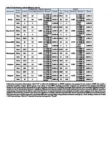
3. Results 3.1. The Poverty Index Table 1 shows all variables used in the construction of the asset index and the result of the PCA. Table 1:
Principal component score
Variable Source of drinking water Piped into dwelling Piped into compound Tap water Well into compound Public well Covered well in the compound Covered public well Spring River Pond Dam Rain Bottle Others
Mean
SD
Component score
Variable
N
0.13 0.13 0.11 0.02 0.06 0.05
0.33 0.33 0.32 0.13 0.24 0.22
0.091 0.030 -0.002 -0.003 -0.021 0.000
7906 7906 7906 7906 7906 7906
0.06 0.12 0.20 0.01 0.04 0.02 0.00 0.05
0.23 0.33 0.40 0.11 0.21 0.14 0.06 0.23
-0.013 -0.028 -0.041 -0.010 -0.024 -0.001 0.020 -0.002
7906 7906 7906 7906 7906 7906 7906 7906
Flush toilet Latrine Ventilated No facility\ bush Others Type of floor material Earth or sand Planks Palm Polished
0.16 0.59 0.08 0.16 0.01
0.37 0.49 0.27 0.37 0.07
0.110 -0.054 0.013 -0.046 0.001
7906 7906 7906 7906 7906
0.56 0.01 0.00 0.01
0.50 0.01 0.02 0.10
-0.100 0.023 -0.001 0.037
7906 7906 7906 7906
Asphalt Ceramic Cement Carpet Other
0.01 0.02 0.37 0.02 0.00
0.09 0.13 0.48 0.13 0.07
0.020 0.041 0.066 0.030 0.017
7906 7906 7906 7906 7906
Type of roof material Grass Tin Iron sheet Concrete Tiles Others Cooking fuel Electricity Gas Bogas Kerosene Coal Charcoal Firewood Other durable goods Has electricity Has radio Has television Has refrigerator Has bicycle Has motorcycle/scooter Has car/truck Has telephone Solar power No. of rooms for sleeping
Sanitation facility
Mean
SD
Component score
N
0.22 0.00 0.65 0.05 0.04 0.02
0.42 0.05 0.48 0.21 0.20 0.13
-0.058 -0.003 0.026 0.052 0.073 -0.010
7906 7906 7906 7906 7906 7906
0.01 0.07 0.00 0.13 0.00 0.16 0.63
0.07 0.26 0.05 0.34 0.02 0.37 0.48
0.023 0.087 0.013 0.043 0.002 0.022 -0.098
7906 7906 7906 7906 7906 7906 7906
0.22 0.77 0.28 0.09 0.29 0.01
0.42 0.42 0.45 0.29 0.46 0.09
0.113 0.042 0.100 0.097 -0.009 0.010
7906 7906 7906 7906 7906 7906
0.09 0.20 0.04 2.18
0.28 0.40 0.19 1.24
0.077 0.105 0.013 0.024
7906 7906 7906 7906
The results of PCA indicate that the first principal component explains 14.3% of the variation in the original variables and each subsequent component explains a decreasing proportion of variance. The screeplot in Figure 1 shows the proportion of variance explained by each principal component and indicates that the first four components would sufficiently explain the original variables.
41
European Journal of Social Sciences – Volume 13, Number 1 (2010) Figure 1: Scree Plot
In the construction of the social economic index, only the factor score (that's the eigenvectors) of the first principal component are used. 3.2. Cross Tabulations
This section presents social economic status cross-tabulated by characteristics of the household; Education, household size, religion, region, age of household head, ethnicity and household own land. The asset index derived from the DHS data was employed to calculate estimate of the headcount poverty index for Kenya. The asset index at the 40-th percentile is employed as the poverty line. Table 2:
Values of Pearson's χ 2 − statistic on cross-classifying demographic characteristics with SES
Explanatory variable Type of place of residence Highest education level Religion Ethnicity Number of household members Age of household head Region
χ 2 − value
df
p-value
1767.69 1397.38 252.094 1146.8649 140.7 33.25 1505.11
1 3 4 14 2 3 7