UNIVERSITE DE GENEVE
CENTRE UNIVERSITAIRE D’INFORMATIQUE COMPUTER VISION AND MULTIMEDIA LABORATORY
Date: 29 June 2004 N° 04.03
TECHNICAL REPORT
Brain-Computer Interface Model: Upper-Capacity Bound, Signal-to-Noise Ratio Estimation, and Optimal Number of Symbols J. Kronegg, S.Voloshynovskiy, and T. Pun
Computer Vision Group Computing Science Center, University of Geneva 24 rue du Général Dufour, CH - 1211 Geneva 4, Switzerland
e-mail:
[email protected]
Submited to EURASIP Journal on Applied Signal Processing (JASP), Special issue on Brain-Computer Interface, 2005.
BRAIN-COMPUTER INTERFACE MODEL: UPPER-CAPACITY BOUND, SIGNALTO-NOISE RATIO ESTIMATION, AND OPTIMAL NUMBER OF SYMBOLS Julien Kronegg, Svyatoslav Voloshynovskiy and Thierry Pun Computer Vision and Multimedia Laboratory, University of Geneva 24 rue General-Dufour, 1211 Geneva 4, Switzerland Phone: +41 22 3797628, fax: +41 22 3797780, email:
[email protected] http://vision.unige.ch/MMI/bci
ABSTRACT The upper capacity bound of a brain-computer interface (BCI) is determined using a model based on Shannon channel theory. This capacity is compared with all bit-rate definitions used in the BCI community (Nykopp, Farwell and Donchin, Wolpaw et al); assumptions underlying those definitions and their limitations are discussed. Capacity estimates using Wolpaw and Nykopp bit-rates are computed for various published BCIs. It appears that only Nykopp's bitrate is coherent with channel theory; Wolpaw's definition leads to an underestimation of the Nykopp's bit-rate and thus should not be used. The usage of a proper bit-rate assessment is motivated and advocated. We also propose an estimation of the typical BCI signal-to-noise ratio, and compute a theoretical optimal number of symbols that is consistent with findings from other researchers. Keywords : brain-computer interface, BCI, upper capacity bound, bit-rate, information theory, channel theory.
1. INTRODUCTION In the brain-computer interface (BCI) paradigm, the user think of a specific notion or mental state (e.g. mental calculation, imagination of movement, mental rotation of objects). EEG data collected from the user are then classified and the mental state identified by the machine. This information can be used to drive a specific application (e.g. virtual keyboard [9], [12], cursor control [38], robot control [33]). During the first 10 years of BCI research (1988-1998), most of the work was focused on discovering new features and classification methods for recognizing mental states, without concentrating too deeply on quantifiable performance comparisons. Results were presented in terms of hit-rates (for cursor control, corresponding to the number of target hit by time unit) or in terms of character-rates (for keyboard applications). It has been further shown that three commonly used BCI design parameters, namely classification speed, number of classes and classifier accuracy are inter-related [12], [18]. Hit-rates or character-rates are therefore not objective measures, since they do not take these three parameters into account.
The first objective BCI performance measure is due to Wolpaw et al in 1998 [38], where the bit-rate was defined on the basis of Shannon channel theory [36] with some simplifying assumptions. Bit-rates commonly reported range from 5 to about 25 bits/minute [39]. For the sake of comparison, it is worth note that a keyboard user can achieve 450-1400 bits/minute (assuming error free typing, 32 possible characters and a typing speed of 90-270 characters/minute, depending on user skill). In this article, we model the BCI as a noisy channel with assumptions that allow to compute the upper capacity bound in term of the amount of reliable information that a BCI user can emit. The present article extends [19] regarding the following issues: various BCIs are compared using both Wolpaw's and Nykopp's bit-rates, the typical signal-to-noise ratio of current BCIs is estimated, and the optimal number of symbols is determined. The article is organized as follows : in Section 2, a review of the noisy channel theory is presented, as a support to the BCI model described in Section 3. Section 4 presents existing bit-rates definitions used in the BCI domain. Discussion of these definitions, and conclusions are presented respectively in Sections 5 and 6. 2. NOISY CHANNEL THEORY A channel is a communication medium that allows the transmission of information from a sender A to a receiver B. Due to imperfections in that medium, the transmission process is subject to noise and B might receive information differing from the one emitted by A. The simplest noisy channel is the additive noise channel where the received signal Y is the sum of an emitted signal X and some independent noise Z here assumed Gaussian (worst case among all noises with the same variance) (see Figure 1). Z ~N(0,σZ2) X Y Figure 1: Model of an additive white Gaussian noise channel. X and Y denote the emitted and received symbols, Z the noise.
Since we deal with real, physical input signals, the input signal energy is limited (which also implies that X has zero mean in order to minimize its energy) : E[X2]≤σX2
The information channel capacity is the quantity of reliable information per channel usage: C = max p ( x ) : E X 2 ≤σ 2 I ( X ; Y )
denoted by p(xi). This leads to the output signal distribution shown in Figure 2. p(y)
X
This capacity is given in bits per symbol and depends on the mutual information between the input signal X and the output signal Y: I(X; Y) = h(Y) - h(Y|X)
… x1
x2
a
xN-1
h ( X ) = ∫ p ( x ) ⋅ log p ( x ) ⋅ dx S
The channel capacity depends on the input signal distribution as well as on the signal-to-noise ratio (SNR) [7]. We consider below three situations with decreasing capacities : continuous input signal, discrete input signal with equiprobable symbols, discrete input signal with non-equiprobable symbols. 2.1 Continuous input signal
N N −1 E X 2 = ∑ xi2 ⋅ p ( xi ) ≤ σ X2 x1 = −σ X 3 N +1 i =1 ⇒ N 3 a = 2 ⋅ σ E [ X ] = ∑ xi ⋅ p ( xi ) = 0 X 2 i =1 N −1 This leads to the capacity CN for discrete equiprobable input signal with N symbols (Eq. 2):
N
CN = ∑
p( y | x ) ∫ p ( y | x ) p ( x ) log p ( y ) dy
+∞
i
i
i =1 y =−∞
h(Y|X) = h(X=x+Z|X=x) = h(N(X=x, σZ2)) = h(Z|X=x)
p ( y | xk ) =
Since X and Z are independents, we have h(Z|X)=h(Z), thus:
)
1 log 2 2 ⋅ π ⋅ e ⋅ (σ X2 + σ Z2 ) bits 2 where the equality holds only for a Gaussian distributed input signal X. We also have the differential entropy of Z: 1 h ( Z ) = log 2 ( 2 ⋅ π ⋅ e ⋅ σ Z2 ) bits 2 This leads to the well known continuous input signal capacity (shown in Figure 3): σ2 1 C = log 2 1 + X2 bits 2 σZ or equivalently as a function of the SNR=10⋅log10(σX2/σZ2):
1 C = log 2 1 + 10 2
SNR 10
1 e 2π σ Z
−
(2)
( y − xk )2 2σ Z2
bits
(1)
j =1
The probability p(y|xi) is the probability that the continuous symbol y is recognized when the symbol xi is sent. The variance σZ2 of the noise Z is given by σZ2 = σX2 ⋅ 10-SNR/10. The capacity CN has to be determined by numerical integration. Figure 3 compares the continuous capacity C (Eq. 1) and the discrete equiprobable capacity CN (Eq. 2). There is an asymptotic difference of 1.53 dB between C and C∞ (the discrete capacity for N=∞), so called shaping loss (which is due to the use of an uniform probability density function instead of a Gaussian one). In all cases, the continuous capacity is greater than the discrete equiprobable capacity. 10
continuous gaussian source
9
N=128
7
N=64
6
N=32
5
N=16
4
N=8
3
N=4 N=3 N=2
2 1
asymptotical capacity for discrete equiprob. signal
2.2 Discrete equiprobable input signal We model the discrete input signal as a Pulse Amplitude Modulation (PAM) signal with N symbols, the noise Z as independent and Gaussian distributed as in the continuous case. All symbols have the same probability p(X=xi)=1/N,
N=512 N=256
8 Information [bits/symbol]
)
(
2
N
The differential entropy of a random variable N(µ, σ2) does not depends on the mean µ: 1 h N µ , σ 2 = log 2 2 ⋅ π ⋅ e ⋅ σ 2 bits 2 The differential entropy of Y depends on its variance Var[Y]=σX2+σZ2, thus:
(
i
p ( y) = ∑ p ( xj ) p ( y | xj )
I ( X , Y ) = h (Y ) − h ( Z )
h (Y ) ≤
y
Since symbols are equiprobable and the noise Z is independent, the values of the symbols xi should be equidistant, in order to jointly minimize the error and the energy: xi = x1 + (i-1)⋅ a. Taking into account the energy constraint allows to determine x1 and a:
A continuous input signal provides a maximal, continuous capacity. Since Y=X+Z and since the value of X is known:
))
xN
Figure 2: Discrete equiprobable signal using PAM.
h() is the differential entropy (entropy of a continuous random variable) and is defined by (S being the support set of the random variable):
( (
Z ~N(0,σZ2)
0 -20
-10
0
10
20 SNR [dB]
30
40
50
60
Figure 3: Comparison of the capacity for Gaussian input C and for discrete equiprobable input CN as a function of the number of symbols N and of the SNR.
2.3 Discrete non-equiprobable input signal In practical situations such as occurring in real BCIs, the input signals xi are often not equiprobable (p(xi)≠1/N). This leads to a capacity (in bits/symbol) approximately bounded by the continuous capacity C and by the entropy of the nonequiprobable source H(X): SNR 1 (3) CN ≤ min log 2 1 + 10 10 ; H ( X ) 2 Eq. 3 can be used to estimate the actual capacity when nonequiprobable input symbols are used. It shows that this capacity varies according to the ordering of the symbols: higher capacities are reached when the most likely symbols have the lowest energy. This clearly has consequences on the design of a BCI protocol, and ought to be taken into account. However, since we are here mainly concerned with an upper capacity bound estimation, we will in the sequel not further elaborate on this aspect.
3. BCI MODEL The BCI is modelled as an additive white Gaussian noise (AWGN) channel (as in [35]), followed by a generic classifier (Figure 4). The input signal X models the brain, a memoryless source discrete of N possible tasks or mental states (classes, e.g. "relax", "left movement", "mental calculation") xi, i=1..N, that are all supposed to have the same a priori probability p(xi)=1/N. As in 2.2, the noise is independent from the input signal, so the N symbols are supposed to have equidistant amplitudes (situation depicted in Figure 2). The Gaussian noise Z models the noise induced by the background activity of the brain. Z ~N(0,σZ2) generic classifier
command
Figure 4: Model of the BCI using an AWGN channel.
The classifier recognizes M output mental states yj, i=1..M where M=N for classifiers without rejection capability and M=N+1 for classifiers with rejection capability, leading to the equivalent lattice scheme shown in Figure 5. The NxM transition matrix p(yj|xi), also called confusion matrix is computed during the classifier training phase. This matrix is composed of the probabilities that a mental state xi is recognized as a mental state yj, and its diagonal elements p(yi|xi) are the classifier accuracies for each class [20], [25]. x1 : xi : xN
Despite the fact that the proposed model does not truly correspond to a real BCI, it allows to define an approximate upper capacity bound CM of the BCI. This upper capacity bound is therefore the one defined for discrete equiprobable inputs (cf. Eq. 2 and Figure 3) but with M instead of N symbols. Since CM is calculated using numerical integration, which is not always practical, it can be written using the continuous capacity C and the entropy of a discrete source with M equiprobable symbols log2M, leading to Eq. 4: SNR 1 CM = min log 2 1 + 10 10 ;log 2 M 2
(4)
This bound is also larger than or equal to the capacity bound for non-equiprobable symbols (Eq. 3) and thus can be considered as the “very upper bound” of the BCI capacity. 4. EXISTING BIT-RATE DEFINITIONS
Y
X
not always memoryless. For example, in average-trial protocols, the user repeats the same symbol a given number of times: the probability that the next symbol is the same than the current one is high. Another example is in text typing applications where the probability of the next letter or group of letter can be predicted with some accuracy. Secondly, the noise is not always Gaussian distributed. For instance, with a BCI that uses as features the energy in specific frequency bands, the noise is distributed according to a Rayleigh law. Thirdly, the symbols a priori probabilities are not always identical (e.g. [14], [25], [26]), this especially in applications where commands are infrequently emitted [2]. Last but not least, the fact that symbol values are most of the time imposed by the used feature might impose additional constraints on xi.
y1 : yj : yN yM
Figure 5: Equivalent lattice network for the BCI model shown on Figure 4. Black arrows depict the diagonal elements p(yi|xi) and grey arrows depict the non-diagonal elements or classification error.
This BCI model however does not truly corresponds to a real BCI application, but more to an ideal BCI. First, the source is
The upper capacity bound obtained according to the BCI model from Section 3 can be compared to the bit-rate definitions used in the BCI domain. If this bound holds, every bitrate definition should lead to a lower bit-rate than from the model. Three bit-rate definitions are in use in the BCI domain. The first one is due to Farwell and Donchin in 1988 [12] when they designed the first BCI. The second definition is due to Wolpaw et al in 1998 [38], and the third one to Nykopp in 2001 [25]. All theses definitions are based on Shannon channel capacity. All bit-rates are indicated in bits/symbol, and can be converted to bits/minute according to: B=V⋅R
[bits/minute]
with V being the classification speed (in symbols/minute) and R the information carried by one symbol (in bits/symbols). The most popular definition is the one from Wolpaw, which is reasonably simple and has often been used [37], [38], [39], [40]. The most generic definition is the one from Nykopp, which corresponds to Shannon channel capacity theory. Wolpaw’s as well as Farwell and Donchin’s definitions are in fact simplifications of Nykopp’s definition.
In order to compare our model with theses bit-rate definitions we assumed the use of Bayes hard-classifier, known to be the optimal hard-classifier if the underlying distribution of the data is known [11] (which is the case since Z is known, see Figure 2). 4.1 Nykopp definition Nykopp’s capacity has been introduced in the framework of the Adaptive Brain Interface (ABI) project [25]. The ABI is a BCI with rejection capacity meaning that no decision is taken if the confidence level of the classification does not exceed a certain threshold. This is modeled by means of an erasure channel where some symbols might be lost during transmission [7]. In summary, Nykopp's capacity is defined by:
First, they supposed that N symbols are recognized if N symbols are emitted by the user. They did not consider additional symbols (such as a "not recognized" mental state) as would be the case for classifiers with rejection, or their equivalent erasure channels. The second assumption is that the symbols (or mental states) all have all the same a priori occurrence probability p(xi)=1/N. The third assumption is that the classifier accuracy P is the same for all target symbols (p(yj|xi)=P for i=j))1. The fourth assumption is that the classification error 1-P is equally distributed amongst all remaining symbols (p(yj|xi)=(1-P)/(N-1) for i≠j). From Eq. 5, all theses assumptions lead to the following simplified bit-rate definition :
C = max p ( x ) I ( X ;Y )
RNykopp = I ( X ; Y ) = H (Y ) − H (Y X )
RWolpaw = log 2 N + P ⋅ log 2 P + (1 − P ) ⋅ log 2 (5)
H ( Y ) = − ∑ p ( y j ) ⋅ log 2 p ( y j ) M
1− P N −1
(6)
5. RESULTS AND DISCUSSION
j =1
p ( y j ) = ∑ p ( xi ) ⋅ p ( y j xi ) N
i =1
H (Y X ) = − ∑∑ p ( xi ) ⋅ p ( y j xi ) ⋅ log 2 p ( y j xi ) N
M
i =1
j =1
The a priori symbol probabilities p(xi) are computed by means of the Arimoto-Blahut optimisation algorithm [17], in order to obtain the best bit-rate or capacity for the underlying channel specified by a given transition matrix. This does not truly correspond to a real BCI because in most cases, the a priori symbols probability is imposed by the application, e.g. [14], [25], [26]. 4.2 Farwell & Donchin definition When designing the first BCI in 1988, Farwell & Donchin introduced a bit-rate definition that did not take the classifier accuracy into account. The assumptions made were of a classifier without rejection (M=N), and perfect (i.e. no classification error). This therefore leads to an identity transition matrix p(yj|xi)=I of size NxN. The mental states were assumed to be equiprobable, thus p(xi)=1/N. From Eq. 5, these assumptions lead to the following bit-rate definition :
RFarwell & Donchin = log 2 N [bits/second] As the classifier is considered to be perfect, this measure does of course not correspond to a real BCI and should therefore not be used in practice. Its main interest is to show the maximum achievable bit-rate for high SNRs. 4.3 Wolpaw definition In 1998, Wolpaw et al suggested that it could be interesting to consider the performance measurement not only from the accuracy point of view but also from the information rate point of view [38]. Using the definition of the information rate proposed by Shannon (see Eq. 5) for noisy channels, they made some simplifying assumptions.
5.1 Bit-rates computation and signal-to-noise ratio estimation Based on the analysis of a number of experimental published protocols and results, it has been possible to compute Wolpaw's and Nykopp's bit-rates in bits/trial and bits/minute (Table 1). The SNR has been graphically determined using Figure 8. For published results that are not specifying the transition matrix needed to compute Nykopp's bit-rate, the transition matrix was simulated using Bayes’ classifier theory and the assumptions proposed in Section 2.2. These computations show that the typical BCI signal-to-noise ratio can be estimated to lie between –6 and 8 dB (see Table 1). An exception is for the first four BCIs of the Table where evoked potentials are used: these BCIs cannot really be compared to the others. The mean bit-rate B of all bit-rates B of Table 1 is only 9 bits/minute, which is very low compared to what is stated in [39] or compared to a typical keyboard bit-rate. 5.2 Determination of the theoretical optimal number of symbols Using the same assumptions as in Section 3 (M-PAM feature, independent Gaussian noise and equiprobable symbols), the transition matrix is computed from Bayes classification theory [11] for varying numbers of symbols and SNRs. The classifier accuracy P is then determined as the maximum of the diagonal of the transition matrix and Wolpaw's bit-rate (Eq. 6) is computed, which leads to Figure 6. This figure shows that for typical BCI signal-to-noise ratios, the optimal number of symbols is 3 or 4, which corresponds to findings from studies on the optimization of the number of symbols [10], [23], [26].
1
The mean or the maximum of the transition matrix diagonal is sometimes used when the classifier accuracy is not the same for all classes [26].
N
P
[6]+ [24]+ UIUC [9]*+ UIUC [12]*+ BerlinBCI [10]+ BerlinBCI [10]+ BerlinBCI [10]+ BerlinBCI [10]+ BerlinBCI [10]+ BerlinBCI [3]+ BerlinBCI [4]+ [30]*+ Graz-BCI [26]+ Graz-BCI [26]+ Graz-BCI [26]+ Graz-BCI [26] Graz-BCI [31]*+ Oxford [28]+ Oxford [34]+ LIINC [27]+ Wadsworth [22]*+ Wadsworth [23]+ Wadsworth [23]+ Wadsworth [23]+ Wadsworth [23]+ ABI [25] ABI [20] ABI [33] Neil Squire [5]* Neil Squire [21]* IM2 [15]* EPFL [13]*
10 36 36 36 2 3 4 5 6 2 2 4 2 3 4 5 2 2 2 2 2 2 3 4 5 3 3 3 2 2 3 3
90.0 80.0 80.0 95.0 87.5 73.1 61.2 51.9 44.8 92.0 72.0 48.0 91.0 78.0 63.0 52.7 85.6 75.0 86.5 73.0 75.0 89.3 77.9 74.7 67.0 69.2 53.1 88.3 98.9 86.6 59.4 80.4
RWolpaw RNykopp SNR V 2.54 3.42 3.42 4.63 0.46 0.47 0.42 0.36 0.31 0.60 0.14 0.18 0.56 0.60 0.46 0.38 0.41 0.19 0.43 0.16 0.19 0.51 0.60 0.78 0.75 0.39 0.12 0.95 0.91 0.43 0.21 0.68
2.51 3.78 3.78 4.62 0.46 0.46 0.42 0.37 0.34 0.60 0.14 0.17 0.56 0.58 0.46 0.43 0.40 0.19 0.42 0.16 0.19 0.51 0.57 0.77 0.77 0.43 0.15 0.96 0.11 0.26 0.20 0.68
17.5 25.0 25.0 30.7 1.2 0.8 0.1 -0.5 -0.9 3 -4.7 -3.9 2.5 2.3 0.6 -0.2 0.5 -3.4 0.7 -4.3 -3.4 1.9 2.2 4.0 3.8 -0.6 -5.8 5.8 7.2 0.9 -3.5 3.1
10.8 11.1 6.9 2.3 13.3 13.3 13.3 13.3 13.3 30.0 120 15.0 9.5 9.5 9.5 9.5 15.0 9.0 5.0 9.0 15.0 10.9 10.9 10.9 10.9 NA 11.0 NA NA NA NA 6
B 27.4 38.0 23.4 10.7 6.1 6.3 5.6 4.8 4.1 17.9 17.3 2.7 5.4 5.7 4.4 3.7 6.1 1.7 2.1 1.4 2.8 5.6 6.6 8.5 8.2 NA 1.3 NA NA NA NA 4.1
Table 1: Computation of the bit-rates for various published BCIs according to Wolpaw's and Nykopp's definitions (Rwolpaw and Rnykopp, in bits/trial). The mean accuracy P (in %) and speed V (in trials/minute) are calculated for a given experiment taking all users into account. The SNR (in dB) is graphically determined using Figure 8. The bit-rate B is computed in bits/minute using Rwolpaw and V for the sake of comparison with others studies. An asterisk (*) denotes articles where the bit-rate definition was not specified; it is assumed in these cases that Wolpaw's definition can be used. A plus (+) denotes articles where the transition matrix was simulated to allow for Nykopp's bit-rate calculation. "NA" stands for "Not Available". 2.5
Wolpaw's definition (Eq. 6) does not hold in a number of practical situations. First, the number of recognized symbols is not always equal to the number of input symbols, like in the ABI of Millán et al where the classifier has a rejection capability [20], [25], [33]. Secondly, the a priori occurrence probability p(xi) is not always the same for all symbols, as has been shown in numerous studies [14], [16], [25], [26], [32]. This is especially true when using the oddball paradigm [1], [2], [9], [12], if the application is a virtual keyboard (due to unequal letter appearance frequencies [9], [12]), or if average-trial protocols are used [1], [9], [12], [18], [24] where the probability of the next symbol depends on the current symbol. Thirdly, the classifier accuracy p(yi|xi) has also been shown to differ between symbols [2], [5], [13], [20], [21], [25], [26], [29], [33]. Finally, the error is not equally distributed over the remaining symbols [2], [5], [13], [20], [21], [25], [26], [33]. Figure 7 compares the bit-rate RNykopp computed using Eq. 5 with the upper-bound capacity CM defined by Eq. 4. In order to allow the comparison between the capacity established by our BCI model and the one provided by this definition, we made the hypothesis that all symbols are equiprobable; the Arimoto-Blahut algorithm was therefore not used. The small difference is due to the fact that a hard-classifier was used in Nykopp’s formalism. Figure 8 presents Wolpaw's bit-rate for higher numbers of symbols and SNRs than Figure 6. In contradiction with the classical result from channel theory, Wolpaw's definition causes a decrease of the bit-rate when the number of symbols increases.
N=6 N=5
10 N=512
9
N=4
2
Information [bits/symbol]
5.3 Discussion of Wolpaw's bit-rate definition
N=256
8
N=3 1.5 N=2
1
0.5
Information [bits/symbol]
BCI group
N=128
7
N=64
6
N=32
5
N=16
4
N=8
3
N=4
2
N=2
1
0 -20
-15
-10
-5
0
5
10
15
20
SNR [dB]
Figure 6: Bit-rates using Wolpaw's definition for SNRs and number of symbols specific to various BCI applications (see Table 1).
0 -20
-10
0
10
20
30
40
50
60
SNR [dB]
Figure 7: Comparison between Nykopp’s bit-rate definition RNykopp (Eq. 5) with hard-classifier (gray line) and the upper capacity bound (black lines) CM (Eq. 4).
10 N=512
9
N=256
Information [bits/symbol]
8
N=128
7
N=64
6
N=32
5
N=16
4
If Wolpaw's definition is used for assessing the performance of a particular BCI, the result will be that this BCI has a lower bit-rate than competitor BCIs assessed using Nykopp's definition, e.g. [6], [18], [26]. More importantly, if this definition is employed to determine the optimal number of symbols (like in [10] or [23], [26]), this could lead to wrong conclusions since for high number of symbols, Wolpaw's bit-rate will always be lower than with smaller number of symbols.
N=8
3
N=4
2
N=2
1 0 -20
-10
0
10
20
30
40
50
60
SNR [dB]
Figure 8 : Bit-rates using Wolpaw's definition (gray line, Eq. 6) and comparison with the upper capacity bound CM (black line, Eq. 4).
Comparing Figure 7 and Figure 8, we can see that for some numbers of symbols and SNRs, Wolpaw's bit-rates are lower than Nykopp's bit-rates. Figure 9 presents the difference between Wolpaw's bit-rate and Nykopp's bit-rate ∆R = RWolpaw − RNykopp. This figure shows values of N and of the SNR for which Wolpaw's bit-rates exceed or not Nykopp's rates. For N>5 symbols, Wolpaw's definition leads to bit-rates that are lower than those obtained according to Nykopp's definition (underestimation). For N=2, both definitions lead to the same bit-rate since the error is distributed on one symbol only. For N