cahier 1797 statistical inference for computable general ... - CiteSeerX

CAHIER 1797

STATISTICAL INFERENCE FOR COMPUTABLE GENERAL EQUILIBRIUM MODELS, WITH APPLICATION TO A MODEL OF THE MOROCCAN ECONOMY Touhami ABDELKHALEK1 and Jean-Marie DUFOUR2

1

Institut national de statistique et d’économie appliquée (INSEA) and Groupe de recherche en économie internationale (GREI), Université Mohammed V, Rabat, Maroc

2

Centre de recherche et développement en économique (C.R.D.E.) and Département de sciences économiques, Université de Montréal

September 1997

_______________ The authors thank André Martens, three anonymous referees and the editor, James Stock, for several useful comments. Our research was conducted under the auspices of the PARADI program which links the C.R.D.E., Université de Montréal, and CREFA, Université Laval, and which is financed as a Center of excellence in international development by the Canadian Agency for International Development. This work was also supported by the Social Sciences and Humanities Research Council of Canada and by the Government of Québec (Fonds FCAR).

RÉSUMÉ Nous étudions le problème de la mesure de l’incertitude des simulations de modèles d’équilibre général calculable (MEGC). Nous décrivons deux approches pour construire des régions de confiance pour les variables endogènes de ces modèles. La première utilise une statistique standard de type Wald. La seconde approche suppose l’existence, pour les paramètres libres du modèle, d’une région de confiance (échantillonnale ou bayesienne) à partir de laquelle des régions de confiance, pour les variables endogènes, sont déduites par une technique de projection. Cette dernière méthode a deux avantages: premièrement, la validité des régions de confiance construites n’est pas affectée par la non-linéarité du modèle; deuxièmement, on peut facilement construire des intervalles de confiance pour un nombre illimité de variables. Nous étudions aussi les conditions sous lesquelles ces régions de confiance prennent la forme d’intervalles et nous montrons que ces méthodes peuvent facilement être utilisées au moyen de méthodes standard de résolution des MEGC. Nous présentons une application sur un modèle de l’économie marocaine qui étudie les effets visant à faire augmenter les rapatriements de capitaux par les résidents marocains à l’étranger. Mots clés :

intervalle de confiance, région de confiance, modèle d’équilibre général calculable, analyse de sensibilité, calibration, projection, Maroc, politique fiscale

ABSTRACT We study the problem of measuring the uncertainty of CGE (or RBC)-type model simulations associated with parameter uncertainty. We describe two approaches for building confidence sets on model endogenous variables. The first one uses a standard Wald-type statistic. The second approach assumes that a confidence set (sampling or Bayesian) is available for the free parameters, from which confidence sets are derived by a projection technique. The latter has two advantages: first, confidence set validity is not affected by model nonlinearities; second, we can easily build simultaneous confidence intervals for an unlimited number of variables. We study conditions under which these confidence sets take the form of intervals and show they can be implemented using standard methods for solving CGE models. We present an application to a CGE model of the Moroccan economy to study the effects of policy-induced increases of transfers from Moroccan expatriates. Keywords :

confidence interval, confidence set, computable general equilibrium models, sensitivity analysis, calibration, projection, Morocco, fiscal policy

1. INTRODUCTION Computable general equilibrium models (CGE) are now widely used to simulate alternative economic policies in both developed and developing countries. For example, Martens (1993) has surveyed not less than 120 models on more than 30 developing countries; for other reviews of the subject, see Shoven and Whalley (1984), Ballard et al. (1985), Manne (1985), Devarajan, Lewis and Robinson (1986), Decaluwé and Martens (1988), and Gunning and Keyzer (1995). Such models are usually non-stochastic and nonlinear. They rely on various assumptions, e.g., on agent behaviour and the choice of exogenous variables (the "closure" of the model). The nature and quality of the data used also influence the results. These usually focus on the reference year of a social accounting matrix (in static models) or on a stationary equilibrium (in dynamic models), and parameter values of behavioral functions. Available data do not typically allow one to estimate CGE models econometrically, and so "calibration" procedures are used to obtain models that can be simulated; see Mansur and Whalley (1984). As emphasized by Wigle (1986), the selection of parameter values in CGE models may be highly subjective and thus raises a natural scepticism on the reliability of the resulting simulations. Parameter values are usually obtained from other studies, possibly on different countries, and may even be entirely subjective. The "elasticities" available from the literature are often only distantly related to the case studied, coming from different countries or time periods than those we are be interested in. Consequently, there is a large uncertainty on these basic ingredients, which gets transmitted to simulation results. As CGE models are almost never estimated by econometric methods [for a rare and notable exception, see however the work of Jorgenson (1984) and his associates], it is difficult to test the assumptions made. Even if model specification is not questioned, the credibility of simulation results is affected by the uncertainty on the parameter values used. Indeed, Mansur and Whalley (1984, pp. 100 and 103) have underscored the crucial character of this stage of the modelization: "The choice of elasticity values critically affects results obtained with these models" and "The set of elasticity values used are critical parameters in determining the general equilibrium impacts of policy changes generated by these models". Further the elasticities or parameters which are most crucial may depend on the experiment conducted; see Pagan and Shannon (1987). The critical role of parameter selection and the difficulties associated with the calibration of CGE models are also discussed in the survey of Shoven and Whalley (1984), who point out that the most widely used procedure for assessing the reliability of the simulations (when an attempt of this sort is made) consists in performing a few alternative simulations with different parameter values: "The procedure generally employed is to choose a central case specification, around which sensitivity analysis can be performed" (Shoven and Whalley, 1984, pp. 1030-1031). This importance of this problem has been recognized by several authors, and various approaches have been proposed for assessing the simulation uncertainty induced by parameter uncertainty; see Pagan and Shannon (1985), Harrison (1986, 1989), Bernheim, Scholz and Shoven (1989), Harrison and Vinod (1992), Wigle (1991), Harrison et al. (1993). The different methods proposed are fundamentally descriptive. They may be classified in five groups: limited sensitivity analysis [Bernheim, Scholz and Shoven (1989), Wigle (1991)], conditional systematic sensitivity analysis [Harrison and Kimbell (1985), Harrison (1986), Harrison et al.(1993)], unconditional systematic sensitivity analysis [Bernheim, Scholz and Shoven (1989), Harrison and Vinod (1992),

2 Harrison, Jones, Kimbell and Wigle (1993)], the "Bayesian" approach of Harrison and Vinod (1992), and the extremal approach of Pagan and Shannon (1985). Limited sensitivity analysis is recommended by Shoven and Whalley (1984) and has been largely used in various applications of CGE models. It simply consists in looking at the sensitivity of the results when a few alternative parameter vectors are considered. Because of the discretionary character of the values selected, this procedure is of course quite unsatisfactory from the point of view of ensuring statistical "objectivity". Conditional systematic sensitivity analysis examines the effect of perturbating one parameter at a time on the solution of the model, and so ignores possible interactions due to simultaneous perturbations and does not provide a criterion for determining the appropriate size of parameter perturbations. Unconditional systematic sensitivity analysis attempts to remedy this situation by considering a parameter grid. Although more satisfactory than previous approaches, this procedure has no statistical foundations and can easily be numerically expensive. The Bayesian approach of Harrison and Vinod relies on a "discretization" of the parameter space on which an a priori distribution is imposed. The latter is then used to compute a distribution, and in particular a measure of central tendency, on the solutions of the model. Finally the extremal approach of Pagan and Shannon is based on a linearization of the model based on the first and second derivatives of the endogenous variables with respect to the uncertain parameters. It is clearly the most rigorous procedure from a statistical viewpoint. In this paper, we shall largely rely on the setup considered by Pagan and Shannon (1985). The reader will find a more detailed description of these different approaches in Abdelkhalek (1994). Note also that Byron (1978) derived standard errors for the coefficients of large social accounting matrices (which are widely used to calibrate CGE models) but those have not apparently been exploited to assess simulation uncertainty in the context of CGE models. In all above studies "calibration" is not explicitly studied. This procedure, largely used in CGE models, is considerably less demanding than econometric analysis, especially because only scant data are required. Mansur and Whalley (1984) and Lau [comment on Mansur and Whalley (1984, pp.127-135)] simply point out that "calibration" also raises difficulties for the reliability of simulation results. Note finally a somewhat different form of calibration has been used and discussed in the "real business cycle" (RBC) literature; see Gregory and Smith (1990, 1991, 1993), Canova (1994), Canova, Finn and Pagan (1992), Fève and Langot (1994), and Kim and Pagan (1995). In this context, alternatives to calibration are usually based on the generalized method of moments and require considerable amounts of data. They are not appropriate for many situations where CGE models are applied, e.g., in developing countries. The distinction between the type of calibration in RBC models versus that in CGE models is really one of definition. In CGE models one tries to find an equilibrium data set, ideally a particular year, to replicate. In RBC and stochastic CGE models one emulate the expected values, especially its first and second order moments. The methods developed in the present may clearly be adapted to measure uncertainty in RBC models. However the peculiarities of such models [e.g., the fact that they are stochastic] require developments that go beyond the scope (and space limitations) of the present paper. In this paper, we study the problem of measuring the uncertainty of CGE model simulations in relation to parameter uncertainty. In Section 2, we describe the general setup considered, which is similar to the one of Pagan and Shannon (1985), and show first that calibration can easily be covered by this setup. Then, in two

3 following sections, we describe two systematic approaches for assessing simulation uncertainty, both of which are based on the classical statistical notion of confidence set. More precisely, we deal with the problem of measuring simulation uncertainty in CGE models by building confidence sets for the endogenous variables of the model, given minimal information on parameter uncertainty in the sense that only one confidence set for the uncertain parameters (not a complete sampling distribution for a parameter estimate or a complete Bayesian prior or posterior distribution) may be sufficient. We study two methods for building such confidence sets. The first one (Section 3) is a direct extension of the approach proposed by Pagan and Shannon (1985). It is based on a standard Wald statistic and assumes that consistent asymptotically normal estimators are available for the free parameters of the model. We describe this method mainly because it is a natural follow-up under the assumptions considered by Pagan and Shannon (1985), although it has not apparently been discussed by previous authors in the context of CGE models. Instead we shall emphasize a second technique, which is both more reliable from a statistical viewpoint and (somewhat surprisingly) easier to implement in the context of CGE models. This second method (Section 4) assumes that a confidence set (sampling or Bayesian) is available for the free parameters. Given this confidence set, we can then obtain valid confidence sets for the variables of interest by a projection technique. This approach has two important advantages: first, the validity of the confidence sets is not affected by the nonlinear character of the model; second, it allows one to easily build simultaneous confidence intervals for an unlimited number of variables of interest (or transformations of these). Further, we study general conditions under which these confidence sets are connected (not a union of disjoint sets) and/or take the form of intervals. Numerical procedures required to apply these procedures are discussed in Section 5. In particular, we show that valid projection-based confidence sets can be obtained easily by using standard methods for solving CGE models [e.g., routines available in GAMS (Brooke et al., 1988)], which make them both conceptually and numerically simple to implement in this context, indeed appreciably more than Wald-type confidence sets. Section 6 presents an application of these procedures to a CGE model of the Moroccan economy built to study the economic effects of policy induced increases of transfers from Moroccans working abroad. In particular, we found that the projection technique was both simple to implement in the case studied and yielded remarkably short and informative confidence intervals for the endogenous variables of interest. We conclude in Section 7. 2. FRAMEWORK In general, a CGE model can be represented by a function M such that

Y ' M(X, $, ()

(2.1) where Y is a vector of m endogenous variables, M is a (typically nonlinear) function which can be analytically complex but remains computable, X is a vector of exogenous (or policy) variables, $ is a vector of p free parameters in a subset ' of ú p, and ( is a vector of k calibration parameters. From a theoretical viewpoint, $ and ( are not fundamentally different. However, they are treated quite differently in CGE models. While the components of $ are parameters (such as elasticities) of the behavioral functions of the model (representing: utility and demand, production and supply, imports, exports, etc), the

4 elements of ( are usually scale or share parameters. The calibration process determines a value of ( which allows the model to reproduce exactly the data of a reference year (possibly adjusted to take into account special circumstances), given the value of the free parameter $. Consequently it is not surprising the selection of these parameters may strongly influence simulation results. In other words, when calibrating a model, we consider the equation Y0 ' M(X0, $, () , where Y0 and X0 are the vectors of endogenous and exogenous variables for a reference year, and solve it for ( (assuming there is a unique solution):

( ' H(Y0, X0, $) / h($) .

(2.2)

ˆ of $ is available, ( is estimated on replacing $ by $ˆ in (2.2). Moreover, ( can usually be When an estimate $ decomposed into subvectors (1 and (2, where (1 does not depend on $ while the second subvector (2 is a function of $, X0 and Y0. We can then write:

(1 ' h1(Y0, X0) ,

(2 ' h2(Y0, X0, $) .

(2.3)

Provided X is known and the deterministic character of the model is not questioned, we can simplify notations and write the model in the more compact form:

Y ' g(X, $) / g($)

(2.4)

where the functions g and g are defined for a particular reference year (after calibration) while g also treats X as given. This formalization of the calibration process will be useful for both the theoretical developments and the implementation of the methods proposed in this paper. Usually the investigator is interested by the effects of alternative policies which are represented by elements of X. The solutions of model M, simulated with different values of X, are then compared and used for decision making. All these solutions depend on the estimate employed for $. Theoretically, this vector should be

ˆ . Unfortunately this is not the case estimated by econometric methods that would yield a covariance matrix for $ in most CGE-based studies. Usually no measure of uncertainty is provided and the only method used to assess this uncertainty consists in looking at the sensitivity of the results to a few parameter configurations. Note also the difficulties associated with the calibration of CGE models are not directly taken into account by the procedures of sensitivity analysis briefly discussed in the previous section. These procedures only consider the estimation of $, not (. In CGE models the dimension of ($), ())) can be quite large and its econometric estimation difficult, if not impossible. Indeed, the number of parameters of a CGE model increases rapidly with the number of sectors and consumers considered. Statistical series at high levels of desaggregation are usually not available, so the number of unknown parameters may easily exceed the number of observations. Calibration may be interpreted as an estimation of ( based on a single year data. It is clear this is only pointwise estimation and the uncertainty of the estimate of $ is not taken into account. We will now propose more systematic approaches for assessing simulation uncertainty. 3. WALD-TYPE CONFIDENCE SETS

5 In this section, we consider a setup identical to the one studied by Pagan and Shannon (1985). In

ˆ of $ is available, $ˆ is based on a sample of size T with an particular, let us suppose an estimate $ T T asymptotically normal distribution:

T($ˆ T & $) 6 N[0, V($)]

(3.1)

T 64

where det[V($)] … 0, with a consistent estimator VˆT($ˆ T) of V($): plim VˆT($ˆ T) ' V($). Under usual regularity T64

conditions [see Gouriéroux and Monfort (1989, volume 2, R.245, p. 556) or Serfling (1980, chap. 3)], we then have: T[g($ˆ T) & g($)] 6 N[0, G($)V($)G($))], where G($) is the (m,p) matrix G($) ' Mg($)/M$) . If T64

rank[G($)] ' m

(3.2)

ˆ ' G($ˆ )Vˆ ($ˆ )G($ˆ )), the variable and setting S T T T T T &1

ˆ [g($ˆ ) & Y] WT(Y) ' T[g($ˆ T) & Y])S T T

(3.3)

is asymptotically distributed like a P2(m) variable when Y = g($). Consequently, the set

ˆ [g($ˆ ) & Y] # P (m) > CY(") ' 6 Y: WT(Y) # P"(m) > ' 6 Y: T[g($ˆ T) & Y])S " T T &1

2

2

(3.4)

where P[P2(m) $ P2"(m)] = ", is a confidence set for Y= g($) with level 1 - " asymptotically. As special cases of CY("), we can also obtain confidence intervals for each element of Y. Since the rank condition (3.2) is not satisfied when m > p, i.e., when there are more endogenous variables than unknown parameters in $, one can build ellipsoidal confidence sets only if the number of endogenous variables is not larger than the dimension of $. Nevertheless, even if m > p, we can still build simultaneous rectangular confidence sets for any number of endogenous variables. Indeed, an individual confidence interval with level 1 - "i (asymptotically) for the i-th endogenous variable Yi = gi ($) is given by

Ci("i) ' 6 Yi : T [gi($ˆ T) & Yi] /T ˆ i T # P"i(1) > 2

where T ˆi

T

2

(3.5)

ˆ , and g($) ' [g ($), g ($), ... , g ($)]) . We then have (for T is the i-th diagonal element of S 1 2 m T

sufficiently large):

P[gi($) 0 Ci("i)] ' 1 & "i ,

i ' 1, ... , m .

(3.6)

Each set Ci("i) is thus a valid confidence interval with level 1 - "i for Yi . It would also be interesting to combine these to obtain a simultaneous confidence set. Unfortunately, individual intervals are not typically independent and the stochastic relationship between the former is difficult to establish. Nevertheless, on using the BooleBonferroni inequality, we see that

6

1 & j P[gi($) ó C i("i)] # P[gi($) 0 Ci("i), i ' 1, ... , k] k

i ' 1

#

Min 1 # i # k

(3.7)

P[g i($) 0 Ci("i)]

for any 1 # k # m, hence

1 & j "i # P[gi($) 0 Ci("i), i ' 1, ... , k] # k

Min 1 # i # k

i'1

(1 & "i ) .

(3.8)

Moreover, if the marginal confidence sets Ci ("i ) all have the same level 1 - "1, we have: 1 & k"1 # P[gi($) 0 Ci("i), i ' 1, ... , k] # 1 & "1 ,

so

that

the

simultaneous

confidence

set

{Y 0 ú : Yi 0 Ci("i), i ' 1, ... , k} has level not smaller than 1-k"1. If we wish to obtain a simultaneous k

confidence set whose level is not smaller than 1 - ", it is then sufficient to build marginal confidence sets with levels 1 - "i , i = 1, ... , k, where ' "i ' " . In particular, we can take "i ' "/k , i ' 1, ... , k . k

i '1

The confidence sets developed in this section are remarkably simple. They suppose however that the function g($) can be approximated reasonably well by linear functions (at least locally) and that the distribution of

T($ˆ T & $) is approximately normal. These limitations are identical with those of the approach of Pagan

and Shannon (1985). 4. PROJECTION-BASED CONFIDENCE SETS Suppose now we have a confidence set C with level 1 - " for $. In other words, C is a subset of úp such that

P[$ 0 C] $ 1 & "

(4.1)

with 0 # " < 1. The region C can be interpreted in two different ways. First, C may be a sampling confidence set obtained by statistical methods (typically, an earlier study), i.e. C = C(Z) is a random subset of úp, based on a sample Z, such that the probability that the fixed vector $ be covered by C(Z) is at least 1-". Second, in other cases, $ itself may be viewed as a random vector and C is a Bayesian confidence set for $. The arguments which follow are applicable irrespective of the interpretation adopted. Denote by g(C) the image of the set C by the function g:

g(C) ' 6 Y 0 ú m : Y ' g($0) for at least one $0 0 C > .

(4.2)

It is then clear that: $ 0 C Y g($) 0 g(C), hence

P[g($) 0 g(C)] $ P[$ 0 C] $ 1 & " , œ $ 0 ' .

(4.3)

This means g(C) is a confidence set for g($) with level at least 1- " [see Rao (1973, section 7b.3, page 473)].1 As the function g is usually nonlinear, the set g(C) may not be easy to determine or visualize. It is not generally an interval or an ellipse. So we may find interesting to simplify its structure. To do this, write

7

g i(C) ' 6 Yi 0 ú : Yi ' gi($0) for some $0 0 C > , i ' 1, ... , m .

(4.4)

It is then clear that: g($) 0 g(C) Y gi($) 0 gi(C) , for i ' 1, ... , m, hence by (4.3),

P[gi($) 0 gi(C), i ' 1, ... , m] $ 1 & " ,

(4.5)

P[gi($) 0 gi(C)] $ 1 & " , i ' 1, ... , m .

(4.6)

The inequality (4.5) shows the sets gi (C), i = 1, . .. , m, constitute simultaneous confidence sets with level 1 " for the components of Y, while (4.6) gives marginal confidence sets with level 1 - " for each component of Y.2 These marginal confidence sets gi(C) are subsets of the real numbers which are simpler to apprehend than the multidimensional set g(C). However, without further assumptions, they do not generally take the form of intervals. To obtain confidence regions that take the form of intervals, consider the values gi L(C) and gi U(C) defined as follows:

g i (C) ' inf6 gi($0): $0 0 C >, L

gi (C) ' sup6 gi($0): $0 0 C >, U

i ' 1, ... , m ,

(4.7)

¯ ' ú ^ {&4,%4} . Then, for all $ 0 where giL(C) and giU(C) take their values in the extended real numbers ú C, gi($) 0 gi(C), i ' 1, ... , m Y giL(C) # gi($) # gi U(C), i ' 1, ... , m, hence L

U

P[g i (C) # gi($) # gi (C), 1 # i # m] $ P[gi($) 0 g i(C), 1 # i # m] $ 1 & " .

(4.8)

The intervals [giL(C), giU(C)], i = 1, ... , m, are thus valid simultaneous confidence intervals (with level 1 - ") for Yi = gi ($), i = 1, ... , m. It is also clear that L

U

P[g i (C) # gi($) # gi (C)] $ 1 & " , i ' 1, ... , m .

(4.9)

We should note here two important points. First, the interval [gi L(C), gi U(C)] is generally larger than gi (C), in the sense that gi(C) f [gi L(C), gi U(C)]. Second, this interval is not necessarily bounded, i.e. we may have gi L(C) = -4 or gi U(C) = +4. It would be interesting to determine conditions under which gi (C) = [gi L(C), gi U(C)], where the interval [giL(C), giU(C)] is closed and bounded. We give such conditions in the three following propositions. If we suppose the function g is continuous [as done by Pagan and Shannon (1985), Wigle (1991) and Bernheim, Scholz and Shoven (1989)] and the confidence set C is compact and/or connected in úp, some interesting properties can be derived.3 More precisely, if we suppose g is continuous and the confidence set C is compact (i.e., C is closed and bounded in úp), then the confidence set g(C) for g($) is also compact. Similarly, each function gi is bounded in C and reaches both a maximum and a minimum at points in C. In this case, we can find vectors $i L and $i U in úp such that gi($Li) ' gi L(C) and gi($Ui) ' gi U(C) i ' 1, ... , m. This result is summarized in the following proposition.

8 PROPOSITION 1: If the function g(.) is continuous and the confidence set C is compact in úp, then the simultaneous confidence set g(C) in úm and the univariate confidence sets gi (C), i = 1, ... , m, in ú are compact. The proofs of the propositions are given in Appendix 1. Thus, when the region C is compact and g is continuous, the values gi L(C) and gi U(C) yield a closed confidence interval for the endogenous variable Yi , for any i = 1, ... , m. However, if we add a connexity assumption on C, further refinements are possible. Indeed if, in addition to the continuity of g, we assume the confidence set C for $ is connected [i.e., one cannot find two open subsets O1 and O2 of úp, both meeting C, such that C f O1 c O2 and C 1 O1 1 O2 = i], the confidence region g(C) for g($) is also connected in úm. Clearly this is the case when C is an ellipsoid. Similarly, the marginal confidence sets gi (C), i = 1, . .. , m are connected in ú. A subset of ú is connected only if it is an interval. Thus under these two conditions, we get confidence sets of the form (-4, gi U(C)), (-4, gi U(C)], (gi L(C) , 4), [gi L(C) , 4), (-4, 4), (giL(C), giU(C)), [giL(C), gi U(C)), (gi L(C), gi U(C)] or [gi L(C), gi U(C)]. This result is in turn summarized by the following proposition. PROPOSITION 2: If the function g(.) is continuous and the confidence set C is connected in úp, then the confidence set g(C) in úm and the univariate confidence sets gi (C), i = 1, . .. , m, in ú are connected. In particular, the sets gi (C), i = 1, . .. , m, are intervals in ú. L

U

Finally,ifinadditiontothecontinuityofg,theregionCisbothcompactandconnectedinú,p wecanseethat gi(C) ' [gi (C), g i (C)]. PROPOSITION 3: If the function g(.) is continuous and the confidence set C is compact and connected in úp , then each one of the univariate confidence intervals gi (C), i = 1, . .. , m, is compact and connected in ú , so L

U

that gi(C) ' [gi (C), g i (C)] , with gi L > -4 and gi U < +4. To illustrate how one can build the intervals [giL(C), gi U(C)] in practice, consider the special case studied by Pagan and Shannon (1985) when the confidence set C is an ellipsoid:

C ' 6 $0 0 ú p: ($ˆ & $0))A($ˆ & $0) # c(") >

(4.10)

ˆ is an estimate of $ and A is the inverse of the "covariance matrix" of $ˆ . Or again, according to a where $ ˆ is the a priori (or a posteriori) mean of $ and A is the inverse of the a priori (or a Bayesian interpretation, $ ˆ . In this case, the confidence set C is both compact and connected. Since g is posteriori) covariance matrix of $ differentiable by assumption, the confidence sets (4.2) and (4.4) are necessarily compact and connected by Propositions 1 and 2 above. In particular, marginal confidence sets for the endogenous variables Yi of the model are closed bounded intervals. The bounds gi L(C) and gi U(C) can be obtained by respectively minimizing and

9 maximizing gi ($) on the set C. Under usual regularity conditions, gi L(C) and gi U(C) may be computed by the Lagrange multiplier method. Setting

‹ ' g i($0) %

8 ˆ [($ & $0))A($ˆ & $0) & c(")] 2

(4.11)

the values of $0 which minimize and maximize gi ($0) under the restriction $ 0 C must satisfy:

Mg i M‹ ' & 8A($ˆ & $0) ' 0 , M$0 M$0

($ˆ & $0))A($ˆ & $0) ' c(") .

(4.12)

Assuming A is non-singular, it follows from (4.12) that the values of $0 which yield gi L(C) and gi U(C), denoted $L(i) and $U(i) , solve the equation:

( C

$(i) ' $ˆ ±

Mgi M$0

)

&1

)A (

Mg i M$0

&

)

c(")

1 2

A &1(

Mgi M$0

) .

(4.13)

Note the bounding values $iL and $iU were also considered by Pagan and Shannon (1985), but without reference to the fact that [gi L(C), gi U(C)] can be interpreted as a confidence interval. The above method of building confidence intervals for the endogenous variables of a CGE model is valid in finite samples in contrast with the Wald-type procedure previously discussed which only has an asymptotic justification. No linear approximation to the (generally nonlinear) relationship between the endogenous variables and $ is made. Of course, the projection technique does not solve by itself the problem of finding a confidence set for $, which in a sampling framework should be obtained by inverting "pivotal" functions [see Dufour (1994)]. But it clearly eliminate possible level distortions associated with the nonlinearity of the function g($). Further, we will see below its numerical implementation is considerably less demanding than one would expect at first sight. 5. ALGORITHMS AND NUMERICAL PROCEDURES In this section, we discuss algorithms for applying the procedures proposed in Sections 3 and 4. They can implemented with various software. The one we used is GAMS-MINOS [see Brooke et al. (1988)] which is by far the most widely utilized by CGE model builders. 5.1. Wald-type procedure

ˆ and Vˆ ' Vˆ ($ˆ ) of $ and V($) To implement the Wald-type procedure, we need estimates $ T T T T

10

ˆ ' G($ˆ )Vˆ ($ˆ )G($ˆ )) . respectively. Under appropriate differentiability assumptions, we can then compute S T T T T T ˆ ) must be evaluated by standard numerical methods. Provided S ˆ is invertible, In general the derivatives G($ T T we get from (3.4) that the set

2 ˆ &1[g($ˆ )&g($)] # P2"(m)> C(") ' 6g($): WT(g($)) # P"(m)> ' 6g($): T[g($ˆ T)&g($)])S T T

(5.1)

is a confidence set with level 1 - " asymptotically for the vector g($). Depending on the value of m, the set C(") can be an interval, an ellipsoid or an hyperellipsoid. When m > p, we can still build simultaneous confidence intervals for the components of Y. For further details on the implementation of this procedure, see Appendix 2. 5.2. Projection procedure Although the theory of the projection technique is fairly simple, numerical methods for applying it to CGE models may be less so. The procedure requires a confidence set C (sampling or Bayesian) in úp such that P[$ 0 C] $ 1 & " , with 0 # " < 1. Since the set C may sometimes cover economically or numerically

inadmissible values (e.g., negative values or values for which the model does not admit a solution), the confidence set C can be restricted only to its admissible values. In a Bayesian setup, this simply involves restricting the support of the prior distribution. For sampling (frequentist) confidence sets, it is easy to see that eliminating (truncating)

inadmissible

values

from

a

confidence

set

does

not

modify

its

level.

If

P[$ 0 C] $ 1 & " and $ 0 C0 , where C0 is a set of admissible values for $ representing a priori information,

we have $ 0 C ] $ 0 C _ C0 , hence

P[$ 0 C] ' P[$ 0 C _ C0] $ 1 & " .

(5.2)

We will now show how one can build valid confidence regions by projection while taking into account the "calibration" of the model. Typically the numerical solution of a CGE model is obtained in two steps. First, the model is "calibrated", i.e. a number of unknown parameters (() are fixed to reproduce the data of the reference year given an estimate of the free parameter vector ($) and the values of the endogenous and exogenous variables of this year. Second, the model is solved with different values of the exogenous variables (e.g., policy variables), given the values of all parameters obtained at the end of the first step. In general, one must solve a set of nonlinear equations. This leads to the following algorithm: (1) compute (ˆ 1 ' h1(Y0, X0) ,

ˆ ; (2) given (ˆ 2 ' h2(Y0, X0, $)

ˆ . In practice, to compute Y, we must solve a $ˆ , X0 , X1 , Y0 , (ˆ 1 and (ˆ 2 , compute Y ' M(X1, (ˆ 1, (ˆ 2, $)

potentially complex nonlinear equation system. Using the GAMS-MINOS program, this can done by maximizing a constant function under the constraints which represent the model. Projection-based confidence sets may be obtained by a modification of the above procedure. To do this, the free parameters and the associated calibrated parameters (2 are treated as endogenous "variables" just like the other endogenous variables Y of the model. More formally, given X0 , X1 and Y0 and a confidence set with

11 level 1 - " for $ (possibly specified by inequalities), we consider the procedure: (1) compute (ˆ 1 ' h1(Y0, X0) ; (2) for each i = 1, ... , m, both maximize and minimize: Yi ' gi(X1, $) ' gi($) subject to the restrictions Y ' M(X1, (ˆ 1, (2, $) , (2 ' h2(Y0, X0, $) and $ 0 C _ C0 .

This nonlinear program must be solved at most 2m times to determine the lower and upper bounds of confidence intervals for each endogenous variable of interest. A good initialization usually accelerates convergence. In particular, good initial estimates of the calibrated parameters and the endogenous variables may be good starting points. The first step of this revised algorithm determines, from data of the social accounting matrix of the reference year (or its equivalent), the values of the calibrated parameters that do not depend on free parameters. Then given X1, the second step treats the free parameters in $ and the associated calibrated parameters (2 as additional variables, while the calibration equations are treated as additional relationships of the model. The inequalities that define the confidence set on $ are also added to the model. The basic structure of the latter is preserved by this program but the parameters ($), ()2)) are specified as "variables". The optimization problem is then solved by minimizing and maximizing each variable of interest. Note the number of times the model is solved depends on the number of variables for which we wish build confidence intervals, not the number of parameters p subject to uncertainty (as happens for the Wald-type procedure). Depending on the values of m and p, one may prefer a procedure over the other. Again the above approach can be applied to any endogenous variable of the model. Simultaneous confidence sets based on Boole-Bonferroni inequalities can also be built for several endogenous variables at a time. 6. APPLICATION TO A CGE MODEL OF THE MOROCCAN ECONOMY To illustrate the procedures proposed in the previous sections, we have built a simple CGE model of the Moroccan economy.4 This model has a fairly standard structure close to the one of models developed by Devarajan, Lewis and Robinson (1990), de Melo and Robinson (1989), Condon, Dahl and Devarajan (1987) and Martin, Souissi and Decaluwé (1993). We will use it to study the economic impact of a 25% increase of transfers from Moroccans working abroad (or workers' remittances), an important source of currency for Morocco. Although this question has intrinsic interest, our first objective here will be to illustrate the methodology proposed. Consequently, we have adopted the most simplified structure that will make clear the procedures. The latter may of course be applied to more complex models. Although simplified, our model will illustrate the methods suggested for assessing the uncertainty associated with the free parameters of the model, which in our case will be foreign trade elasticities.

6.1. A simplified CGE model of the Moroccan economy

12 The model studied here is of the "1-2-3" type representing the economy of a single country, Morocco in this case, with two sectors and three goods. Each one of the two sectors produces one good. The first one EX is deemed for export and not sold on the domestic market. The second good D is produced and sold on the domestic market. The third good M is imported and not produced domestically. The assumption that Morocco is a "small country" is preserved so that the prices of exports and imports are exogenous. More precisely, to model foreign trade, we have used a formalization based on recent theories of product differentiation as described by de Melo and Robinson (1989, 1992). It is clear this modelization can have an important influence on the results of policy simulations especially when the latter directly affect the foreign sector. In this theory, an imperfect substitutability between goods is assumed (Armington hypothesis), in contrast with the classical assumption of perfect substitutability between local and imported goods. More precisely, we have a composite good Q consumed on the domestic market, which is a function of imports M and the domestically produced good D with constant elasticity of substitution (CES) between M and D. The representative consumer selects a combination of M and D which minimizes total expenditure given the two corresponding prices pM and pD and the level Q. The Armington formulation of this CES function is given by

Q ' B * M&

D

% (1 & *) D & D

&

1 D

' B * M

F & 1 F

% (1 & *) D

F & 1 F

F F & 1

,

(6.1)

where F ' 1/(1 % D) is the constant elasticity of substitution between imported and domestic goods, B is a constant which depends on measurement units and * is a weighting parameter. In our terminology, following usual calibration procedures for this type of function in CGE models [see Mansur and Whalley (1984)], B and * are calibrated parameters while F (or D) is a free parameter that needs to be estimated before calibration. The first order equilibrium condition for this problem is given by the equality of the price ratio between the two goods and the marginal rate of substitution between imported and domestic goods or equivalently:

M/D ' */(1 & *)

F

pD/pM

F

.

(6.2)

The prices pM and pD are endogenous. The price pC of the composite good is determined by the equations:

pC Q ' pM M % pD D ,

p M ' pwm (1 % tm) E

(6.3)

where pwm is the international price of imports, tm the duty rate on imports, and E the nominal exchange rate which can be fixed in some formulations of the model. Exports are modeled in a comparable way. Again, in contrast with the standard small economy hypothesis, we suppose there is product and market differentiation. It is still assumed that Morocco is a "pricetaker" on the international market, but domestic producers can choose to direct their supply, denoted Xs, either towards the domestic market or towards exports depending on relative prices. Since there is a quality difference between products sold locally and exported products, a constant elasticity transformation function (CET) between these two products is specified. Exports come from local production (not the composite good), so the direct

13 content in import of exports is taken to be zero. However, their indirect content through intermediate consumption may not be void. Producers maximize their income given the technological constraint represented by the transformation function, i.e., they maximize

p X s ' pD D % p E EX

(6.4)

subject to the constraint

X ' B E ( EX s

R

% (1 & () D

1 R R

.

(6.5)

The price of exports pE, the price of the domestic good pD as will as the composite supply price p are endogenous. pE is evaluated in national currency and defined by the expression

pE (1 % te) ' pwe E

(6.6)

where pwe is the international price of exports, E the nominal exchange rate and te the duty rate on exports. Again, to help interpretation, we define S ' 1/(R & 1) , or R ' (1 % S)/S . As before, BE is a scale parameter, ( a weight coefficient, and S a constant elasticity of transformation between exports and the domestic good. BE and ( are calibrated parameters while S (or R) is a free parameter for which an estimate is required. The maximization of (6.4) subject to (6.5) yields the condition

EX / D ' (1 & ()/(

S

pE/p D

S

.

(6.7)

This way of modelling foreign trade, studied in detail by de Melo and Robinson (1989) and Devarajan, Lewis and Robinson (1990), is widely used in CGE models.5 It appears more realistic than the classical assumption of perfect substitutability between goods. The two functions CES and CET are sufficiently easy to manipulate in analytic derivations and calibration, even though a free parameter is introduced by each function. The functions are homogenous of degree one with respect to their arguments. Given a hypothesis of factor full employment, the CET function defines a concave production possibility frontier between exports and sales on the domestic market. Equations (6.1)-(6.7) all belong to the model. Overall, the model has 30 equations (including Walras law), 42 variables, 2 free parameters, 10 calibration parameters and 5 tax parameters. To solve it model, we need to treat as exogenous 13 of the 42 variables. By the small country assumption, it is natural to take the prices of exports and imports as exogenous. Six categories of transfers between agents (government to firms, government to households, government to the rest of the world, rest of the world to households, rest of the world to government, firms to the rest of the world), government expenditures, total labor and capital are also taken as exogenous. This corresponds to a classical "closure" of the model, in the sense that investment adjusts itself to total available saving [see Decaluwé, Martens and Monette (1988)], which could be contrasted with Keynesian, Kaldorian and Johansen-type closures. To complete the closure, the balance of the current account is treated as

14 exogenous (the nominal exchange rate remains endogenous) and the price pc of the composite good is taken as numeraire (fixed by definition). 6.2. Deterministic calibration of the model To calibrate the model described above, we used a social accounting matrix of the Moroccan economy constructed by G.R.E.I. (1992) and econometric estimates of the two free parameters (the foreign trade elasticities F and S). To show how this is done, consider the Armington-type model for imports described above. To calibrate the parameters which appear in this function, we first need an estimate of the substitution elasticity F. Then, using the first order condition (6.2), the data on the values Q0 , M0 , D0 , pD and pM of the reference year, 0

0

and a normalization convention on the prices of the same year,6 we can write

M0/D0

1 Fˆ

' */(1 & *) pD /pM , 0

(6.8)

0

from which we get an estimate of *:

pM /pD M0/D0

*ˆ '

1 Fˆ

0

0

1% pM /pD M0/D0 0

1 Fˆ

/ h21(Fˆ ).

(6.9)

0

An estimate of the scale parameter B follows on using equation (6.1):

Bˆ ' Q0 /

*ˆ M0

Fˆ & 1 Fˆ

ˆ D % (1 & *) 0

Fˆ & 1 Fˆ

Fˆ Fˆ & 1

/ h22(F) ˆ .

(6.10)

In equations (6.9) and (6.10), the crucial role played by the free parameter for determining the other parameters is clear. In this case we usually have D0 > M0 what entails h21(ˆF) is an increasing function of Fˆ . When the elasticity of substitution is small, which is the case for developing countries like Morocco, *ˆ tends to zero and numerical problems show up in solving the model. We can proceed in a similar way for the parameters of the export function which depend on the free parameter S. Further details are given in Abdelkhalek (1994). To calibrate and simulate this model, we need estimates of the foreign trade elasticities F and S. No earlier estimates of such parameters for Morocco appear to be available in the literature. The closest work is the one of Khan (1975) and Stern, Francis and Schumacker (1976), who estimated import and export elasticities with respect to their relative price, as opposed to the substitution and transformation elasticities which appear in our model. Further, the work of Khan (1975) leads to elasticities which are essentially zero for Morocco over the period 1951-69, so we estimated the needed elasticities from Moroccan data over a more recent period. The two required elasticities were estimated simultaneously from Moroccan data covering the period 1962 to 1992. An econometric analysis of structural change in the two estimated equations (relating the

15 logarithms of the ratios D/M and E/D to the logarithms of the corresponding price ratios and a measure of overall economic activity) led us to divide the sample into two more homogeneous subperiods (1962-1972 and 19731992). The two estimated equations are given in Appendix 3. Without going into the details of this econometric analysis, which is not the purpose of this paper, note the two equations have contemporaneously correlated disturbances, so the latter were estimated as a set of seemingly unrelated regressions (SURE): shocks that affect exports may also affect imports and vice-versa, hence the correlation between the disturbances. We obtained in this way the following estimates for (S, F) for the subperiod 1962-1972, with the corresponding asymptotic covariance matrix:

ˆ ' 0.392957 , Fˆ ' 1.432371 ; Eˆ ' S T T

0.185303

& 0.017096

& 0.017096

0.024113

.

(6.12)

Of course, given the very small sample size on which these estimates are based, the usual large sample distributional theory may not be very reliable here, and the resulting confidence sets should be interpreted with caution. Given the available data, these appeared to be the best that could be obtained. Using these estimates of the free parameters of the model, we can then calibrate the other parameters on the basis of the reference year and simulate the model. The latter were performed with the GAMS-MINOS program.

6.3. A simulation In general, CGE models are built to study the effects of various economic policies or changes in other exogenous variables (X) of the model. Given a change in X, the model is solved for a new equilibrium. We will study here the effect of a 25% increase in transfers from the rest of the world to households in Morocco. These transfers consist mainly of repatriations by Moroccan workers abroad, an important source of foreign currency for Morocco. Indeed, the latter country receives more currency from this source than from phosphate exports and tourism. These transfers of income have increased during the 1980's due to returns of emigrants and to various public policies encouraging fund repatriations. As these transfers may take several channels, they are difficult to measure statistically. In particular they can go through formal channels or take the form of liquidities brought during holidays, settlements between compatriots or even purchases of imported goods. The first of these elements is the only one measured by official balance of payments statistics, which shows a regular progression at an annual rate of 22% between 1970 and 1990.7 This evolution appears to corroborate a positive reaction to various incentives put forward by public authorities. Because of the importance of these repatriations, it is of interest to study their economic impact on the Moroccan economy. Although our first objective here will be to illustrate the methods proposed above, our general equilibrium simulations will also provide useful information for economic policy. The transfers have direct effects on household income, and indirect effects on consumption,

16 saving, investment and government revenue. The simulation which follows studies these aggregate effects. The results of the simulation are displayed in Table 1. They show that the increased influx of currency raises household income YM and saving SM, consumption CM, and thus total demand originating from households, both for the composite good Q and the domestic good D. Since the structure of the model, and especially its closure, does not allow an increase in supply (added value VA or intermediate consumption CI), the price pD of domestic goods increases leading to an increase of imports M (because of their substitutability with domestic goods). The currency influx decreases the nominal exchange rate E, i.e. leads to an appreciation of the national currency, which in turn decreases exports EX and increases imports M. As imports increase more in value than exports decrease and duty rates are higher on imports, government receipts increase. Furthermore, due to the raise of household income, direct taxes increase, government saving SG follows, and the government deficit decreases. The current balance account (saving from the rest of the world) is exogenous in this model and thus remains unchanged. All savings increase or remain fixed. Aggregate investment IT, given the closure of the model, increases and puts additional pressure on internal demand and imports. All these trends are symptoms of what is known as the "Dutch disease". The reactions of the endogenous variables of the model, especially imports, exports and internal demand for the domestic good depend on the substitutability between the different goods represented by the elasticities S and F. Indeed the smaller these elasticities the larger the effects of the shocks simulated here. The results in Table 1 only give point estimates of the endogenous variables associated with given elasticity estimates and exogenous variables. Any serious analysis should look at the robustness of the results to parameter uncertainty. The procedures proposed above allow one to build confidence sets for the endogenous variables of the model, and we will now give such confidence sets for the endogenous variables of most interest. - Wald-type confidence sets As there are only two free parameters in this model, confidence sets of ellipsoidal type may be built only for two variables at a time. We can however obtain Wald-type confidence intervals for all the variables of the model. We shall concentrate on six of these variables: exports (EX), imports (M), government saving (SG), aggregate investment (IT), internal demand for the domestic good (D), and the nominal exchange rate (E). Table 2 gives the partial derivatives of these six endogenous variables with respect to the two free parameters, which are the source of the uncertainty. These derivatives were evaluated by numerical methods (as described in Appendix 2) using symmetric parameter perturbations with h ' $ˆ kT/1000 . Given these, we can build marginal confidence intervals for the endogenous variables of interest. Table 3 presents such intervals (with level 95%) for the endogenous variables under the new vector of exogenous variables, the difference with respect to the reference year value and the difference in percentage. We see from these that the effect of the 25% increase in transfers is clearly positive (at 5% level) for three variables (M, SG, IT) and negative for another one (E), while

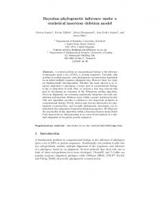
17 the intervals for EX and D include zero indicating that these effects are not statistically significant (although these intervals also cover values that may economically sizable). All the intervals are fairly precise in the sense that the difference between the upper and lower bounds (the range) are always less than 4% of the corresponding level, even less than 1% for IT and D. Tables 2 and 3 also give confidence interval construction for variables taken individually. In the case of this model, ellipsoidal simultaneous confidence sets can be obtained for pairs of endogenous variables. For the sake of illustration, we give in Figure 1 a 95% confidence ellipsoid for the changes of public saving SG and aggregate investment IT. We see from the shape of this ellipse that the changes in SG and IT are positively associated, which is not surprising. We also report on the same figure Boole-Bonferroni 95% simultaneous confidence intervals (rectangular confidence region) which are easier to understand but are less precise.

- Projection-based confidence sets The simultaneous estimations of the two foreign trade elasticities S and F by the SURE procedure yields a covariance matrix which can be used to build a confidence set for the vector $ ' (S, F)). This confidence set can be rectangular if we ignore the covariance between the estimators of the two foreign trade elasticities. Interestingly, this approach also allows one to use estimates which are not based on the same data or for which a covariance matrix is not available. In the case considered here, we have a covariance matrix and so we can build an ellipsoidal confidence set for S and F. For illustrative purposes, we present below results based on rectangular and ellipsoidal confidence sets for $. Throughout the confidence level is 95%. The rectangular confidence set is obtained by simply estimating S and F separately (through two regressions) and then building confidence intervals CS and CF for S and F from these regressions. To ensure that the resulting rectangle has the desired coverage probability, we build confidence intervals CS and CF with levels 1 - "1 and 1 - "2 respectively, where " = "1 + "2. In contrast with the SURE approach considered below, this method does not make any assumption on the form of the dependence between the errors in the two equations. This is due to the fact the level " = "1 + "2 is obtained through the Boole-Bonferroni inequality which holds irrespective of the nature of the dependence between the two separate regressions used; for further discussion of such methods, see Dufour and Torrès (1997). More precisely, we take "1 = "2 = "/2 = 0.025 and find the intervals: ˆ & t(" ; 8) s ˆ , S ˆ % t(" ; 8) s ˆ , C ' S S

CF '

1

S

1

S

Fˆ & t("1 ; 6) sFˆ , Fˆ % t("1 ; 6) sFˆ

(6.14)

where sSˆ and sFˆ are the usual standard error estimates for Sˆ and Fˆ , t("1 ; -4 and giU(C) < +4. Q.E.D.

22

APPENDIX 2: WALD-TYPE PROCEDURE ALGORITHM The main difficulty in the implementation of the Wald-type procedure is to compute the derivatives G($ˆ T) . This can be done as follows. After a first solution of the model has been obtained for the reference year with $ ' $ˆ T and the initial values of the exogenous variables, we solve the model a second time (base solution) with a new set of exogenous variables (which may represent a different policy) but keeping the same coefficient vector $ˆ T . We then need to evaluate the matrix G($ˆ T) of the derivatives of Y at the base solution. This can be done by considering small perturbations, symmetrical or not, of each component of $ˆ T . In the case of symmetrical perturbations, we need to solve the model 2p times (in addition to the two basic simulations), while only p solutions are required for asymmetrical perturbations. The relative precision of the two procedures depends on the shape of the function g(.). In both methods, parameter perturbations should be very small and applied to one parameter at a time. For each perturbed parameter vector, the model is then solved (with the same set of exogenous variables). The difference between two corresponding perturbed solutions (in the symmetrical case) or between each perturbed solution and the base solution is then used to evaluate each partial derivative. More precisely, G($ˆ T) is evaluated as follows (in the case of symmetrical perturbations): (1) solve the model with $ ' $ˆ T and calibrate it to reproduce the reference year according to equations Y0 ' M(X0, $, () and (2.2); (2) compute the new equilibrium under the new exogenous variables vector X1, which yields the base solution: Y ' g(X1, $ˆ T) ; (3) for each k = 1, ... , p, consider k k two modified $ vectors, the first obtained by changing component $ˆ T of $ˆ T to $ˆ T % h (the other k k components remaining the same) and the second one by changing $ˆ T to $ˆ T & h where h is small; k the value of h may be a fixed fraction of $ˆ T or of its standard deviation; (4) solve the model with these modified parameter vectors (and the new exogenous variables vector); calibrated parameters which are functions of free parameters are of course modified after each perturbation of a free parameter; (5) for k = 1, ... , p, evaluate the partial derivatives with the formula: Mg )

M$k

(X1, $ˆ T) '

1 k p 1 k p g(X1, $ˆ T, .., $ˆ T % h, .., $ˆ T) & g(X1, $ˆ T, .., $ˆ T & h, .., $ˆ T)

2h

.

(A.1)

The latter algorithm allows one to evaluate the matrix G($ˆ T) for any values of p and m. Since VˆT ˆ . However, because of the rank condition (3.2) is known, we can then compute easily the matrix S T which cannot to be satisfied when m > p (i.e., when there are more endogenous variables than free parameters) simultaneous confidence sets of ellipsoidal type can be constructed only when the number of endogenous variables is at most equal to the number of free parameters. When p = 2 for example, simultaneous confidence sets for pairs of endogenous variables may be so obtained.

23

APPENDIX 3: ESTIMATION OF FOREIGN TRADE ELASTICITIES To obtain the free parameters S et F, we estimated the following pair of equations from M D

ln

' "0 % F ln

PD PM

% "1 ln (PIB) % u1 ,

(A.2)

annual Moroccan data: ln

E D

' (0 % S ln

PE PD

% (1 ln (PIBW) % u2 .

(A.3)

The data come from the International Monetary Fund [International Financial Statistics (I.F.S.), 1992 and January 1994] and the variables are defined as follows: M: Index of imports, line 73 of I.F.S. (1985 = 100); D: Index of domestic consumption (1985 = 100); PD : Wholesale price index, line 63 of I.F.S. (1985 = 100); PM : Price index of imports, line 75 of I.F.S. (1985 = 100); PIB : Real gross domestic product in billions of 1985 dirhams, line 99b of I.F.S.; E: Index of exports, line 72 of I.F.S. (1985 = 100); PE : Price index of exports, line 74d of I.F.S. (1985 = 100); PIBW: Index of gross domestic product of industrialized countries, line 110 of I.F.S.(1985 = 100). The parameters of (A.2) and (A.3) were estimated first equation by equation (by least squares) and then as a SURE system, using Micro TSP (version 6.0). The results of the estimations are displayed in Table A.1.

24 Table A.1: Estimation of foreign elasticities* Independent

OLS

SURE

variables

Constant

ln(PD/PM)

ln (M/D)

ln (E/D)

ln (M/D)

ln (E/D)

1.80681

1.54106

1.81084

3.00096

(0.7172)

(1.0832)

(0.5329)

(0.8615)

1.26371

----

1.43237

----

(0.2653) ln(PIB)

-0.47815

(0.1553) ----

(0.1649) ln(PE/PD)

----

-0.45754

0.69138

----

(0.7417) ln(PIBW)

----

-0.47823

Sample size

----

-0.78371 (0.1821)

9

11

9

9

0.8132

0.6260

0.7983

0.7390

s (S.E. of reg.)

0.0578

0.0768

0.0601

0.0711

D-W

2.5010

1.4767

2.2939

1.2114

R2

*

0.39296 (0.4305)

(0.19844) **

----

(0.1272)

Standard errors are given in parentheses. Because of missing data, the numbers of observations differ across equations (9 observations for 1964-72, and 11 observations for 1962-72). **

25 REFERENCES Abdelkhalek, Touhami, "Inférence statistique pour modèles de simulation et modèles calculables d'équilibre général: théorie et applications à un modèle de l'économie marocaine," Ph.D. Thesis, Université de Montréal, (1994). Ballard, Charles L., Don Fullerton, John B. Shoven, and John Whalley, "A General Equilibrium Model for Tax Policy Evaluation," (Chicago: University of Chicago Press, 1985). Bernheim, Douglas B., John K. Scholz, and John B. Shoven, "Consumption Taxation in a General Equilibrium Model: How Reliable are Simulation Results?," Technical Report, Departement of Economics, Stanford University (1989). Brooke, A., David Kendrick, and A. Meeraus, GAMS: A User's Guide (Palo Alto, CA: The Scientific Press Redwood City 1988). Byron, R.P., "The Estimation of Large Social Account Matrices," Journal of the Royal Statistical Society, series A, 141 (1978), 359-369. Campbell, Bryan, and Jean-Marie Dufour, "Exact Nonparametric Tests of Orthogonality and Random Walk in the Presence of a Drift Parameter," International Economic Review, 38 (1997), 151-173. Canova, Fabio, "Statistical Inference in Calibrated Models," Journal of Applied Econometrics, 10 (December 1994), Supplement, S123-S144. Canova, Fabio, M. Finn, and Adrian R. Pagan, "Evaluating a Real Business Cycle Model," in Hargreaves C. (ed.) Nonstationary time series analysis and co-integration (Oxford: Oxford University Press 1992). Centre Marocain de Conjoncture, "Les transferts des TME: tendances et comportements," Lettre du C.M.C. nº7/8, (october-november 1991). Condon, Timothy, H. Dahl, and Shantayanan Devarajan, "Implementing a computable general equilibrium model on GAMS: The Cameroon Model," Technical Report, Development Research Department, Economics and Research Staff, World Bank (1987). Decaluwé, Bernard, and André Martens, "CGE Modeling and Developing Economies: A Concise Empirical Survey of 73 Applicaitons to 26 Countries," Journal of Policy Modeling, 10 (1988), 529-568. Decaluwé, Bernard, André Martens, and Marcel Monette, "Macro Closures in Open Economy CGE Models: A Numerical Reappraisal," International Journal of Development Planning Literature, 3 (2) (1988), 6980. de Melo, Jaime, and Sherman Robinson, "Productivity and externalities: models of export-led growth," The journal of International Trade & Economic Development 1 (1992), 41-67. de Melo, Jaime, and Sherman Robinson, "Product Differentiation and General Equilibrium Models of Small Economies," Journal of International Economics 27 (1989), 47-67 .Devarajan, Shantayanan, Jeffrey D. Lewis, and Sherman Robinson, "Policy Lessons from Trade-Focused Two Sector Models," Journal of Policy Modelling 12 (1990), 625-657. Devarajan, Shantayanan, Jeffrey D. Lewis, and Sherman Robinson, "A Bibliography of Computable General Equilibrium (CGE) Models Applied to Developing Countries," Technical Report No. 224, Harvard University, Cambridge, Massachusetts (1986). Dufour, Jean-Marie, "Nonlinear Hypotheses, Inequality Restrictions and Non-Nested Hypotheses: Exact

26 Simultaneous Tests in Linear Regressions," Econometrica 57 (1989), 335-355. Dufour, Jean-Marie, "Exact Tests and Confidence Sets in Linear Regression with Autocorrelated Errors," Econometrica 58 (1990), 475-494. Dufour, Jean-Marie, "Some Impossibility Theorems in Econometrics, with Applications to Structural and Dynamic Models," Technical report, C.R.D.E., Université de Montréal (1994). Forthcoming in Econometrica. Dufour, Jean-Marie, and Jan F. Kiviet, "Exact Inference Methods for First-order Autoregressive Distributed Lag Models," Technical Report, C.R.D.E., Université de Montréal (1994). Forthcoming in Econometrica. Dufour, Jean-Marie, and Jan F. Kiviet, "Exact Tests for Structural Change in First-Order Dynamic Models," Journal of Econometrics, 70 (1996), 39-68. Dufour, Jean-Marie, and Olivier Torrès, "Union-Intersection and Sample-Split Methods in Econometrics with Applications to SURE and MA(1) Models," in D. Giles and A. Ullah (eds.), Handbook of Applied Economic Statistics (New York: Marcel Dekker, 1997) forthcoming. Fève, Patrick, and François Langot, "The RBC Models Through Statistical Inference: An Application with French Data," Journal of Applied Econometrics 10 (December 1994), Supplement, S11-S35. Gouriéroux, Christian, and Alain Monfort, Statistique et modèles économétriques, Volumes 1 and 2 (Paris: Economica 1989). Gregory, Allan W., and Gregor W. Smith, "Calibration as Estimation," Econometric Reviews 9 (1990), 57-89. Gregory, Allan W., and Gregor W. Smith, "Calibration as Testing: Inference in Simulated Macroeconomic Models," Journal of Business and Economic Statistics 9 (1991), 297-303. Gregory, Allan W., and Gregor W. Smith, "Statistical Aspects of Calibration in Macroeconomics," in Maddala, G.S., Rao, C.R., and Vinod, H.D., (eds.), Handbook of Statistics, Volume 11 (Amsterdam: Elsevier Science Publishers B.V. 1993). Groupe de Recherche en Economie Internationale (G.R.E.I.), "La Matrice de Comptabilité Sociale du Maroc de 1985," Monographie 1, Centre d'études stratégiques, Faculté des sciences juridiques, économiques et sociales, Université Mohammed V Rabat (1992). Gunning, Jan W., and M.A. Keyzer "Applied General Equilibrium Models for Policy Analysis," in J. Behrman and T. Srinivasan (eds.), Handbook of Development Economics, Vol. 3A, 2026-2107 (Amsterdam: North-Holland 1995). Harrison, Gleen W., "A General Equilibrium Analysis of Tarrif Reduction," in T.N. Srinivasan and J. Whalley, (eds.), General Equilibrium Trade Policy Modelling (Cambridge, MA: MIT Press 1986). Harrison, Glenn W., "The Sensitivity Analysis of Applied General Equilibrium Models: A Comparison of Methodologies," Technical Report, Department of Economics, University of New Mexico (1989). Harrison, Glenn W., Richard Jones, Larry J. Kimbell, and Randall Wigle, "How Robust Is Applied General Equilibrium Analysis?," Journal of Policy Modeling 15 (1993), 99-115. Harrison, Glenn W., and Larry J. Kimbell, "Economic Interdependance in the Pacific Basin: A General Approch," in J. Piggot and J. Whalley, (eds.), New Developements in Applied General Equilibrium Analysis (Cambridge: Cambridge University Press 1985). Harrison, Glenn W., and Hrishikesh D. Vinod, "The Sensitivity Analysis of Applied General Equilibrium Models: Completly Randomized Factorial Sampling Designs," Review of Economics and Statistics 79

27 (1992), 357-362. International Monetary Fund, International Financial Statistics (1992, 1994). Jorgenson, Dale W., "Econometric Methods for Applied General Equilibrium Analysis," in H.E. Scarf and J.B. Shoven (eds.), Applied General Equilibrium Analysis (Cambridge: Cambridge University Press 1984). Khan, Moshin S., "Import and Export Demand in Developing Countries," IMF Staff Papers 21 (1975), 678-693, International Monetary Fund, Washington D.C. Kehoe, Timothy J., "Regularity and Index Theory for Economies with Smooth Production Technologies," Econometrica 51 (1983), 895-919. Kim, K., and Adrian R. Pagan, "The Econometric Analysis of Calibrated Macroeconomic Models," in M.H. Pesaran and M.R. Wickens (eds.), Handbook of Applied Econometrics: Macroeconomics, 356-390 (Oxford: Blackwell 1995). Kiviet, Jan F., and Jean-Marie Dufour, "Exact Tests in Single Equation Autoregressive Distributed Lag Models," Journal of Econometrics (1997) forthcoming. Manne, Alan S., "On the Formulation and Solution of Economic Equilibrium Models," Mathematical Programming Study 23 (1985), 1-22. Mansur, A., and John Whalley, "Numerical Specification of Applied General Equlibrium Models: Estimation, Calibration, and Data," in H.E. Scarf and J.B. Shoven (eds.), Applied General Equilibrium Analysis (Cambridge: Cambridge University Press 1984). Martens, André, "La politique économique de développement et les modèles calculables d'équilibre général: un mariage à la progéniture abondante," Collection G.R.E.I., Volume 1, 96-119, (Morocco: Rabat 1993). Martin, Marie-Claude, Mokhtar Souissi, et Bernard Decaluwé, "Les modèles calculales d'équilibre général: les aspects réels," Technical Report, École PARADI de Modélisation de politiques économiques de développement, volume 2, C.R.E.F.A., Université Laval et C.R.D.E., Université de Montréal (1993). Miller, R.G., Simultaneous Statistical Inference, Second edition (New York: Springer-Verlag 1981). Pagan, Adrian R., and J.H. Shannon, "How Reliable are ORANI Conclusions?," Economic Record 63 (1987), 33-45. Pagan, Adrian R., and J.H. Shannon, "Sensitivity Analysis for Linearized Computable General Equilibrium Models," in J. Piggot and J. Whalley, (eds), New Developpements in Applied General Equilibrium Analysis (Cambridge: Cambridge University Press 1985). Rao, Calyampudi R., Linear Statistical Inference and Its Applications, Second edition (New York: John Wiley and Sons 1973). Royden, H.L., Real Analysis, Second edition, (New York: MacMillan 1968). Serfling, Robert J., Approximation Theorems of Mathematical Statistics (New York: John Wiley and Sons 1980). Shoven, John B., and John Whalley, "Applied General Equilibrium Models of Taxation and International Trade: an Introduction and Survey," Journal of Economic Literature 22 (1984), 1007-1051. Stern, Robert M., J. Francis, and B. Schumacker, Price Elasticities in International Trade: An Annotated Bibliography (London: Macmillan 1976). Wigle, Randall, "The Pagan-Shannon Approximation: Unconditional Systematic Sensitivity in Minutes,"

28 Empirical Economics 16 (1991), 35-49. Wigle, Randall, "Summary of the Panel and Floor Discussion," in T.N. Srinivansan and J. Whalley (eds.), General Equilibrium Trade Policy Modeling (Cambridge: MIT Press, 323-354 1986).

29 TABLES AND FIGURE Table 1: Simulation results for a 25% increase of transfers from the rest of the world to households in Morocco Variable

Reference year value

Value after simulation

Variable change

SAM 1985 in value

in %

VA

116858.000

116858.000

0.0000

0.0000

CI

121584.800

121584.800

0.0000

0.0000

pD

1.000

1.00602

0.00602

0.60200

pC

1.000

1.000

0.0000

0.0000

pM

1.21134

1.18247

-0.02887

-2.38331

pE

0.98966

0.96607

-0.02359

-2.38365

E

1.000

0.97617

-0.02383

-2.38300

CM

83829.100

85948.75722

2119.65722

2.52855

IT

35122.800

35666.55332

543.75332

1.54815

M

42806.000

44761.86308

1955.86308

4.56913

EX

32198.000

31867.92374

-330.07626

-1.02515

D

209847.000

210168.7960

321.79600

0.15335

Q

261699.700

264363.111

2663.41100

1.01774

YM

102093.100

104674.571

2581.47100

2.52855

YG

23402.700

23709.12414

306.42414

1.30935

TAXM

9046.700

9234.58631

187.88631

2.07685

TAXE

333.000

321.73096

-11.26904

-3.38410

SM

14116.000

14472.92953

356.92953

2.52855

SG

-4677.600

-4371.17586

306.42414

6.55088

30 Definitions of variables in Table 1 VA :

Value added in volume

M:

Imports in volume

CI :

Intermediate consumption in volume

EX :

Exports in volume

pD :

Price of domestic good

D:

Internal demand for domestic good

pC :

Price of composite good

Q:

Demand for composite good in volume

pM :

Domestic price of imported good

YM :

Houshold income

pE :

Price of exported good

YG :

Government income

E:

Nominal exchange rate (price of

TAXM :

Taxes on imports

foreign currency in dirhams)

TAX :

Taxes on exports

CM :

Household consumption in value

SM :

Household saving

IT :

Aggregate investment in value

SG :

Government saving

Table 2: Partial derivatives of endogenous variables of interest with respect to free parameters Variable

1

Reference value

Value after

Partial derivative

Partial derivative

1

SAM 1985

simulation

with respect to S

with respect to F

EX

32198.00

31867.92374

-704.70814873

175.60394618

M

42806.00

44761.86308

-625.08111575

282.41984793

SG

-4677.60

-4371.17586

-55.51498001

168.39212746

IT

35122.80

35666.55332

-13.84375390

224.97662966

D

209847.00

210168.7960

688.37048328

-168.60157041

E

1.00

0.97617

0.01272404

0.01047215

After 25% increase of transfers from the rest of the world to Moroccan households.

31 Table 3: Marginal Wald-type confidence intervals with level 95% for six endogenous variables Varia-

Confidence interval

Confidence interval for difference with

ble

reference year (1985) value

Difference in value

Difference in %

Lower

Upper

Lower

Upper

Lower

Upper

bound

bound

bound

bound

bound

bound

Range

EX

31257.500

32478.347

-940.4999

280.3474

-2.9210

0.8707

3.7917

M

44206.248

45317.478

1400.2481

2511.4780

3.2711

5.8671

2.5960

SG

-4448.946

-4293.405

228.6535

384.1947

4.8883

8.2135

3.3252

IT

35594.208

35738.899

471.4077

616.0989

1.3422

1.7541

0.4119

D

209572.824

210764.768

-274.1761

917.7681

-0.1307

0.4374

0.5681

E

0.9657824

0.9865576

-0.0342176

-0.013442

-3.4218

-1.3442

2.0776

32 Table 4: Confidence intervals with level 95% for six endogenous variables endogenous A. Projection from a rectangular confidence set for the parameters Variable

Confidence interval

Confidence interval for difference with reference year (1985) value

Difference in value

Difference in %

Lower bound

Upper bound

Lower bound

Upper bound

Lower bound

Upper bound

Range

EX

30609.184

31966.332

-1588.8164

-231.6680

-4.9345

-0.71951

4.21501

M

43561.513

44908.459

755.5117

2102.4609

1.7650

4.91160

3.14664

SG

-4699.347

-4290.609

-21.7466

386.9907

-0.4649

8.2733

8.73818

IT

35223.041

35772.746

100.2383

649.9453

0.28539

1.85049

1.56510

D

210073.700

211402.950

226.7031

1555.9063

0.10803

0.74145

0.63342

E

0.9506900

0.9893900

-0.04931

-0.010610

-4.93100

-1.06100

3.87000

B. Projection from an ellipsoidal confidence set for the parameters Variable

Confidence interval

Confidence interval for difference with reference year (1985) value

Difference in value

Difference in %

Lower bound

Upper bound

Lower bound

Upper bound

Lower bound

Upper bound

Range

EX

31095.856

31963.886

-1102.1445

-234.1133

-3.42302

-0.72711

2.69592

M

44044.210

44904.419

1238.2110

2098.4180

2.8926

4.90217

2.00955

SG

-4515.478

-4293.113

162.1221

384.48730

3.46592

8.21976

4.75383

IT

35470.860

35769.392

348.0586

646.5898

0.99098

1.84094

0.84996

D

210076.000

210926.200

229.0000

1079.2031

0.10913

0.51428

0.40515

E

0.9647500

0.9858600

-0.035250

-0.014140

-3.52500

-1.41400

2.11100

33

Figure 1 : Simultaneous confidence sets for VSG and VIT (level = 95%)